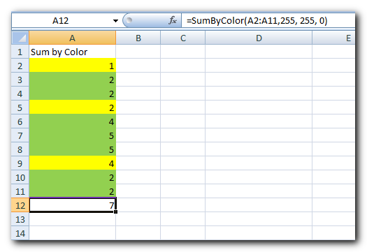
Recently some of our subscribers have requested us to share a VBA code that can sum the cells by its color. To help our subscribers and developers, we are sharing 2 codes that be used to sum the cells with specific color and returns the total sum of the matching color cells
Public Function SumByColor(rng As Range, Red As Long, Green As Long, Blue As Long) As Double

    'Variable declaration
    Dim dblSum As Double
    Dim rngCell As Range

    'Loop throught each cell in the range
    For Each rngCell In rng
        'Checking and sum color
        If rngCell.Interior.Color = RGB(Red, Green, Blue) Then
            If IsNumeric(rngCell.Value) = True Then
                dblSum = dblSum + rngCell.Value
            End If
        End If
    Next

    'Return the value
    SumByColor = dblSum

End FunctionPublic Function SumByColor(rng As Range, ColorCell As Range) As Double
'Variable declaration
Dim dblSum As Double
Dim rngCell As Range
'Loop throught each cell in the range
For Each rngCell In rng
'Checking and sum color
If rngCell.Interior.Color = ColorCell.Interior.Color Then
If IsNumeric(rngCell.Value) = True Then
dblSum = dblSum + rngCell.Value
End If
End If
Next
'Return the value
SumByColor = dblSum
End Function
Step 1: Open the Excel file in which you want to copy this code
Step 2: Press Alt+F11 to open VBA editor
Step 3: Insert a new module from Insert > Module menu
Step 4: Paste the code in the module
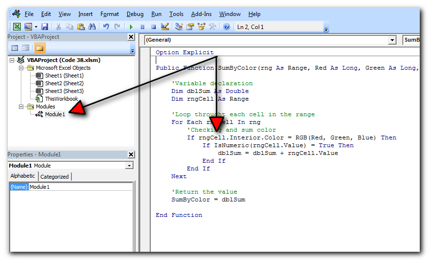
Step 5: Now you are ready to use this code as Excel Function/Formula
Step 6: Type the formula in the cell where you want to get the sum specific colored cells
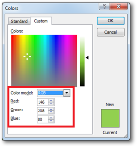
First Code Example: =SumByColor(A2:A11,146, 208, 80)
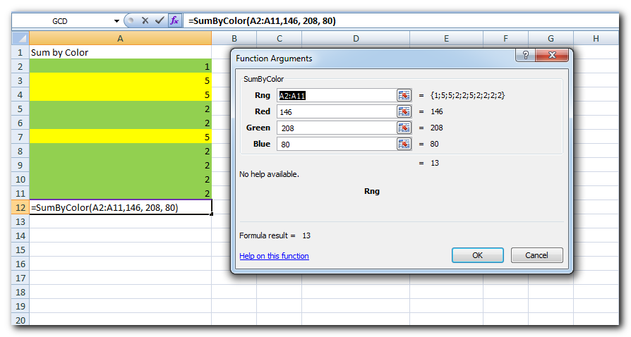
The first parameter of the formula is the range from which you want to sum the specific color cells. The second, third and fourth parameters are RGB code of the color.
Second Code Example: =SumByColor(A2:A11,A3)
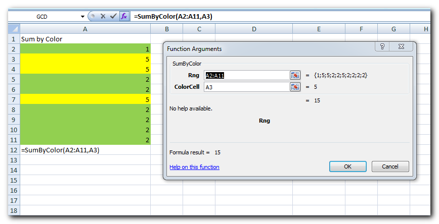
The first parameter of the formula is the range from which you want to sum the specific color cells. The second parameter is the cell from which you want to compare the color.
Step 1: Select the cell which contain the color you want to use
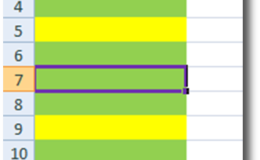
Step 2: Right click and select ‘Format Cells…’
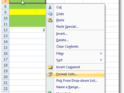
Step 3: In the Format Cells dialog box go to ‘Fill’ tab and click on ‘More Colors…’
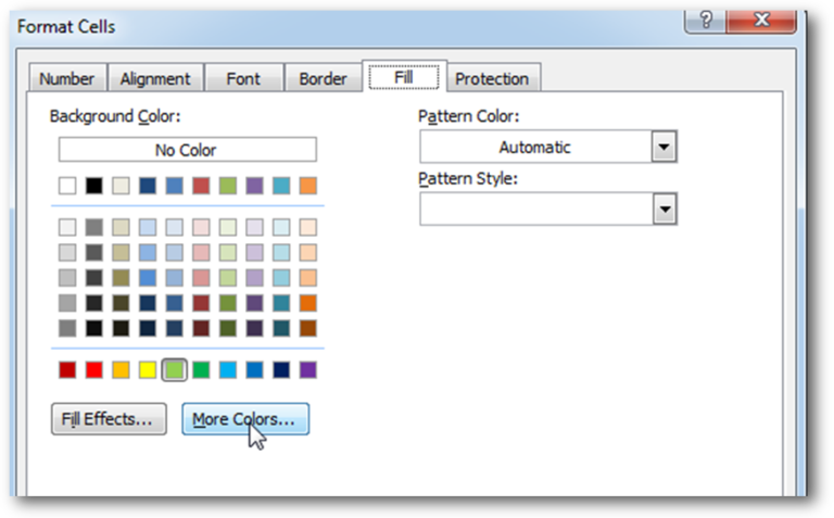
Step 4: That’s all, in the ‘Color’ dialog box, you can view the RGB (Red, Green, Blue) codes of the color
Thanks for reading the article, subscribe us to get more VBA tricks
Through formatting the cells, you can make your Excel data more beautiful and easier to understand. If you record a macro to add borders to Excel range, you will notice that it generates 30 plus lines of code for just a small work. Here we are sharing one line of code which does the same thing.

Table of Content How does testing help? How should I test my tool or application? How does Dummy Data Generator tool helps in testing? How do I use this tool? From many years I have…
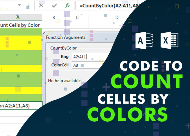
Have you ever felt that Microsoft should have added a formula in Excel which can count the cells based on specific color? I have seen many code requests to share a VBA code that can count the cells by its color. To help our subscribers and developers, we are sharing 2 codes that be used to count the cells with specific color and returns the count of the matching color cells.
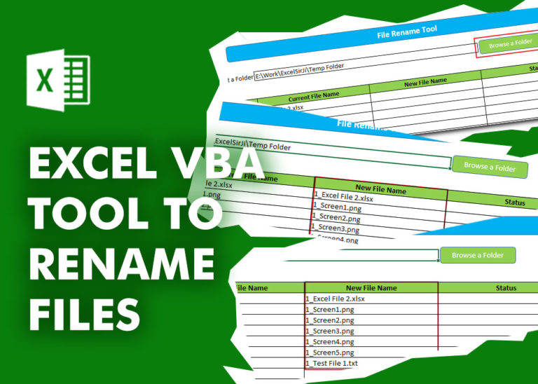
Free File Renamer Tool – Quickly Rename files batch using Excel VBA Here is another help code and tool for programmers to rename files. You can use this tool for renaming all files available in…

VBA CODE TO HIDE MENU RIBBON IN MS ACCESS In MS Access, there are multiple ways to protect your code or tool from un-authorized access and edits. Some developers prefers to hide MS Access ribbons…

This guide explains the basics of Excel’s Advanced Filter and shows you how to use it to find records that match one or more complicated conditions.
If you’ve read our previous guide, you know that Excel’s regular filter offers different options for filtering text, numbers, and dates. These options work well for many situations, but not all. When the regular filter isn’t enough, you can use the Advanced Filter to set up custom criteria that fit your exact needs.
Excel’s Advanced Filter is especially useful for finding data based on two or more complex conditions. For example, you can use it to find matches and differences between two columns, filter rows that match another list, or find exact matches with the same uppercase and lowercase letters.
Advanced Filter is available in all Excel versions from 365 to 2003. Click the links below to learn more.
Hi,
How to Count (D71) CONDITIONALLY FORMATTED RED COLOR CELL only (D40:D70)?
Pls guide…
Thanks
If you want to count from single cell then formula will be =SumByColor(D71,256,0,0)