How to color alternate rows in Excel: highlight every other row
This tutorial shows you how to color alternate rows in Excel and automatically highlight every other row or or column in your worksheets. You will also learn how to use Excel’s banded rows and columns and find some helpful formulas to shade rows based on value changes.
Using alternating colors for rows in Excel is a common way to make data easier to read. While it’s simple to manually highlight rows in a small table, it can be very time-consuming in larger tables. A better approach is to automatically alternate the colors of rows or columns, and this article will show you how to do it quickly
Table of Contents
How to color alternate rows in Excel
When it comes to shading every other row in Excel, many experts will suggest using conditional formatting. This method requires some time to figure out a clever combination of the MOD and ROW functions.
However, if you’d rather not spend a lot of time on this task—like using a sledgehammer to crack a nut—you can use the built-in Excel table styles as a quick and easy alternative to create zebra-striped tables
Highlight every other row in Excel using banded rows
The quickest and easiest way to shade rows in Excel is by using predefined table styles. Tables have many benefits, including automatic filtering, and they automatically shade rows with different colors. To turn a range of cells into a table, just select your range and press Ctrl + T together.
Once you do this, the odd and even rows in your table will automatically be shaded with different colors. The best part is that this automatic shading will keep working even when you sort, delete, or add new rows to your table.
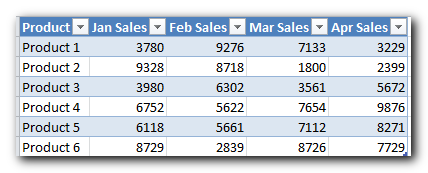
If you’d rather have alternate row shading only, without the table functionality, you can easily convert the table back to a usual range. To do this, select any cell within your table, right click and choose Convert to Range from the context menu.
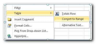
Note. After performing the table-to-range transformation, you won’t get the automatic color banding for newly added rows. Another disadvantage is that if you sort the data, your color bands will travel with the original rows and your nice zebra stripe pattern will get distorted.
As you can see, converting a range to table is a very easy and quick way of highlighting alternate rows in Excel. But what if you want a bit more?
How to choose your own colors of row stripes
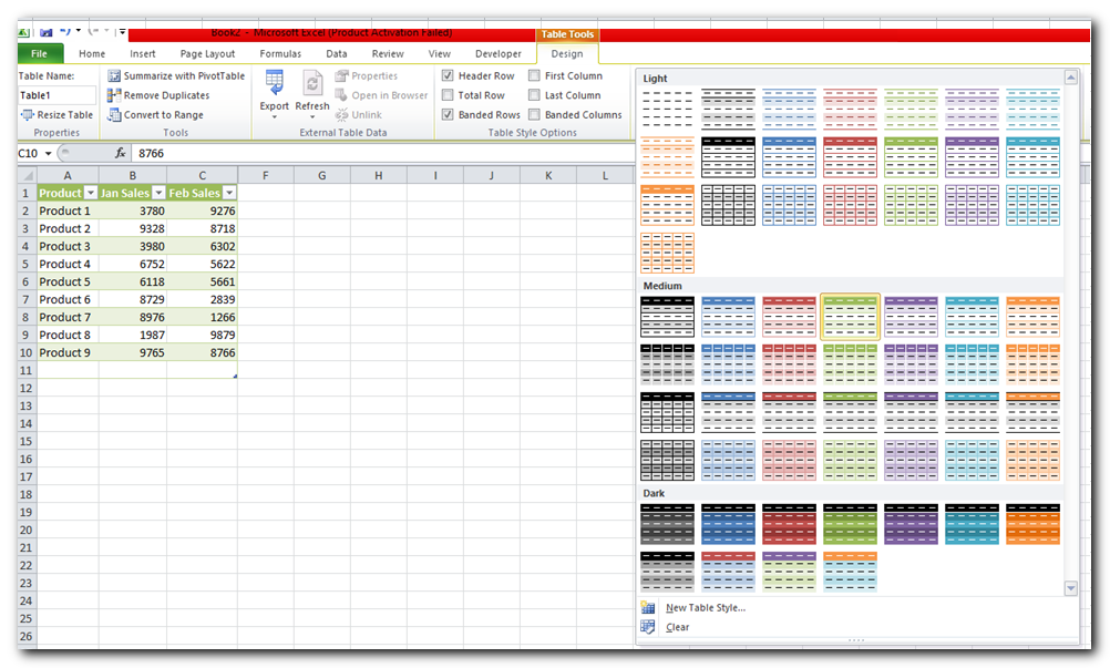
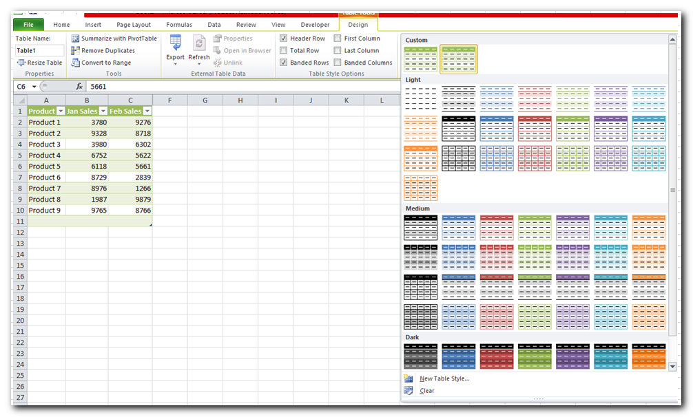
If you don’t like the default blue and white pattern of an Excel table, there are many other colors and patterns to choose from. Just select your table or any cell in it, go to the Design tab, and look for the Table Styles group to pick your favorite colors.
You can use the arrow buttons to scroll through the available table styles or click the More button to see all the options. When you hover your mouse over any style, it shows up on your table right away, so you can see how the banded rows will look.
How to highlight a different number of rows in each zebra line
If you want to highlight a different number of rows in each stripe—for example, shading 2 rows in one color and 3 in another—you will need to create a custom table style. If you’ve already turned a range into a table, follow these steps:
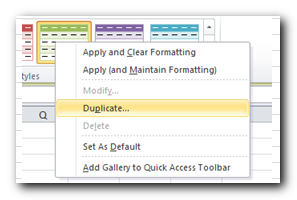
- Go to the Design tab, right-click on the table style you want to use, and choose Duplicate
- In the Name box, enter a name of your table style.
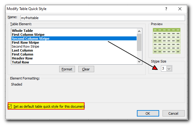
- Select “First Row Stripe” and set the Stripe Sizeto 2, or to some other number you want.
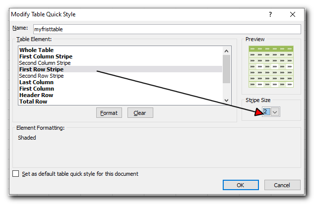
- Select “Second row stripe” and repeat the process.
- Click OK to save your custom style.
- Apply the newly created style to your table by selecting it from the Table Styles gallery. Your custom styles are always available at the top of the gallery under Custom
Note: Custom table styles are stored only in the current workbook and therefore are not available in your other workbooks. To use your custom table style as the default table style in the current workbook, select the “Set as default table style for this document” check box when creating or modifying the style.
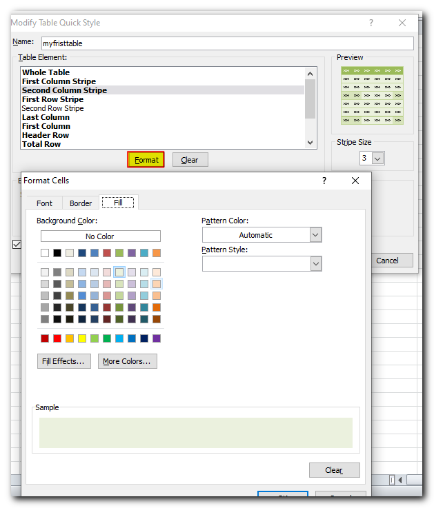
If you’re not satisfied with the style you created, you can easily change it. Just right-click your custom style in the Styles Gallery and select Modify from the menu. This is your chance to be creative! You can set any font, border, and fill styles on the different tabs, and even choose gradient stripe colors, as shown in the screenshot below.
Remove alternate rows color in Excel with a click
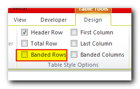
If you no longer want to have color banding in your Excel table, you can remove them literally in a single click. Select any cell in your table, go to the Design tab and uncheck the Banded rows option.
As you can see, Excel’s predefined table styles offer many features for alternating row colors and creating custom banded row styles. These styles will work well in many situations. However, if you want something more specific, like shading entire rows based on a change in value, you will need to use conditional formatting.
Alternate row color shading using Excel conditional formatting
Conditional formatting is a bit more complex than the Excel table styles we just talked about. However, it has a big advantage: it gives you more creative freedom to design your worksheet exactly how you want it in each case. Later in this article, you will find some examples of Excel formulas for alternating row colors:
Highlight every other row in Excel using conditional formatting
We will start with a simple MOD formula that highlights every other row in Excel. You can get the same result using Excel table styles, but the main advantage of conditional formatting is that it works for ranges too. This means your color banding will stay the same even when you sort, insert, or delete rows in the data range that your formula applies to.
You create a conditional formatting rule in this way:
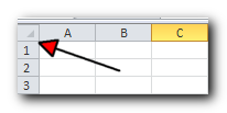
- Select the cells you want to shade. To apply the color banding to the entire worksheet, click the Select All button in the top left-hand corner of your spreadsheet.
- Switch to the Home tab> Styles group and click Conditional Formatting > New Rule…
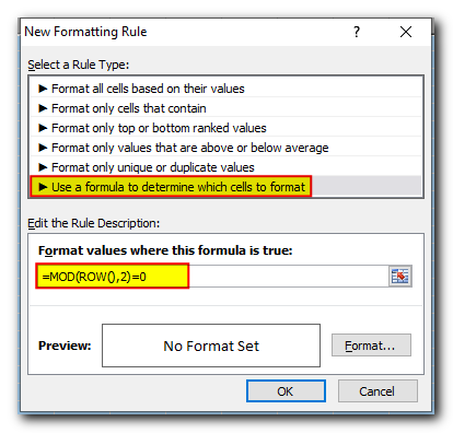
- In the New Formatting Rule window, choose “Use formula to determine which cells to format” option and enter this formula: =MOD(ROW(),2)=0
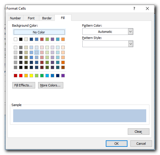
- Then click the Format button, switch to the Fill tab and select the background color that you want to use for the banded rows.
At this point, the selected color will appear under Sample. If you are happy with the color, click OK.
- This will bring you back to the New Formatting Rulewindow, and you click OK one more time to apply to color to every other of the selected rows.
And here’s how the result looks like in my Excel 2010:
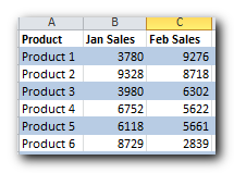
If you’d rather have 2 different colors instead of white lines, then create a second rule using this formula:
=MOD(ROW(),2)=1
And now you have odd and even rows highlighted with different colours
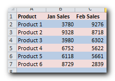
That was pretty easy, right? Now, I’d like to briefly explain the syntax of the MOD function because we will use it in some slightly more complex examples.
The MOD function gives you the remainder after dividing a number by another number.
For example, =MOD(4,2) returns 0 because 4 divides evenly by 2 (with no remainder).
Now, let’s look at what our MOD function does in the example we used earlier. We combined the MOD and ROW functions like this: =MOD(ROW(),2). The syntax is simple: the ROW function gives the row number, then the MOD function divides that number by 2 and returns the remainder. When we apply this formula to our table, it gives us the following results:
Row No. | Formula | Result |
Row 2 | =MOD(2,2) | 0 |
Row 3 | =MOD(3,2) | 1 |
Row 4 | =MOD(4,2) | 0 |
Row 5 | =MOD(5,2) | 1 |
Do you see the pattern? It’s always 0 for even rows and 1 for odd rows. And then we create the conditional formatting rules telling Excel to shade odd rows (where the MOD function returns 1) in one color and even rows (that have 0) in another color.
Now that you know the basics, let’s look into more sophisticated examples.
How to alternate groups of rows with different colors
You can use the following formulas to shade a fixed number of rows, no matter what content they have:
Odd row shading (highlight the 1st group and every other group):
=MOD(ROW()-RowNum,N*2)+1<=N
Even row shading (highlight the 2nd group and all even groups):
=MOD(ROW()-RowNum,N*2)>=N
In these formulas, RowNum refers to the first cell with data, and N is the number of rows in each banded group
Tip: If you want to highlight both even and odd groups, then simply create 2 conditional formatting rules with both of the above formulas.
How to shade rows with 3 different colors
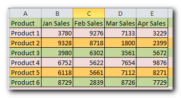
If you think your data will look better with rows shaded in three different colors, create three conditional formatting rules using these formulas:
- To highlight the 1st and every 3rd row:
=MOD(ROW($A2)+3-1,3)=1 - To highlight the 2nd, 6th, 9th, etc.:
=MOD(ROW($A2)+3-1,3)=2 - To highlight the 3rd, 7th, 10th, etc.:
=MOD(ROW($A2)+3-1,3)=0
Make sure to replace A2 with the reference to your first cell with data.
The resulting table will look similar to this in Excel:
The TRANSPOSE function in Excel is used to change rows into columns, or columns into rows. It helps you switch the direction of a selected range from horizontal to vertical, or the other way around.
The function only needs one input:
TRANSPOSE(array)
An array is the group of cells you want to switch.
When transposed, the first row of the original group becomes the first column in the new group, the second row becomes the second column, and so on.
How to alternate row colors based on a value change
This task is similar to the one we just discussed about shading groups of rows, but here, each group may have a different number of rows. I think it will be easier to understand with an example.
Imagine you have a table with data from different sources, like regional sales reports. You want to shade the first group of rows for the first product in Color 1, the next group for the second product in Color 2, and so on. Column A, which lists the product names, can act as the key column or unique identifier.

To alternate row shading based on change of value, you’d need a bit more complex formula and an additional column:
- Create an additional column over the right side of your worksheet, say column F. You will be able to hide this column later.
- Enter the following formula in cell F2 (assuming that row 2 is your first row with data) and then copy it across the entire column:
=MOD(IF(ROW()=2,0,IF(A2=A1,F1, F1+1)), 2)
The formula will fill down column F with blocks of 0 and 1, every new block staring with the Product name change.
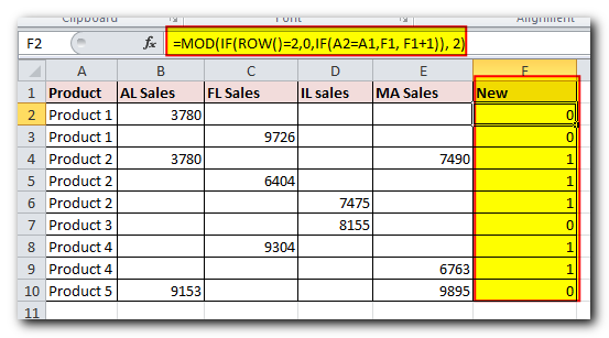
- And finally, create a conditional formatting rule using the formula =$F2=1. You can add a second rule =$F2=0if you want a second color to alternate blocks of rows, as shown in the screenshot:
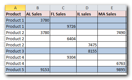
Alternating column colors in Excel (banded columns)
Actually, shading columns in Excel is very similar to alternating rows. If you understood everything we talked about earlier, this part will be easy for you! 🙂
You can apply shading to columns in Excel by using either:
Alternate column colors in Excel with table styles
- You start with converting a range to a table (Ctrl+T).
- Then switch to the Design tab, remove a tick from Banded rows and select Banded columns instead.

- Voila! Your columns are shaded with the default table colors.
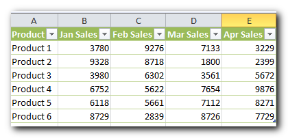
If you want nicer colors, you can pick any other pattern from the Table Styles Gallery.
I hope you now feel confident about applying color banding in Excel to make your worksheets look nice and easier to read. If you want to alternate row or column colors in a different way, feel free to leave a comment, and we can work on it together. Thank you for reading!


