Excel EXPAND function: To grow array to specified number of rows and columns
This tutorial explains a new Excel 365 function that helps you make an array bigger to the size you want by filling it with a chosen value.
Do you need to expand an array to a certain number of rows or columns so all similar arrays in your worksheet are the same size? In Excel 365, you can do this with just one simple formula. Say hello to the new EXPAND function, which lets you grow an array to any size you need
Table of Contents
Excel EXPAND function
The EXPAND function in Excel is designed to pad an array with a value of your choice to the specified row and column dimensions.
The syntax includes the following arguments:
Array (required) – the original array.
Rows (optional) – the number of rows in the returned array. If omitted, new rows are not added, and the columns argument must be set.
Columns (optional) – the number of columns in the returned array. If omitted, new columns are not added, and the rows argument must be set.
Pad_with – the value to fill new cells with. If omitted, defaults to #N/A.
EXPAND function availability
Currently, the EXPAND function is available in Excel for Microsoft 365 (Windows and Mac) and Excel for the web.
How to use the EXPAND function in Excel
To make an array bigger, use the EXPAND formula like this:
- Array: Enter a range of cells or an array of values from another formula.
- Rows and Columns: Type in positive numbers larger than the current number of rows and columns in the array. These numbers set the final size of the array, not just the extra rows or columns to add. In each formula, you must set either rows or columns (or both). If you skip one, Excel will use the size of the original array for that part.
- Pad_with: Choose a value to fill the new cells. If it’s text, put it in double quotes (e.g., “Hello”). If it’s a number, just type it (e.g., 5). If you don’t enter a value, Excel will fill the new cells with #N/A.
Since EXPAND is a dynamic array function, you only need to enter it in one cell. It will automatically fill the required number of rows and columns based on your formula.
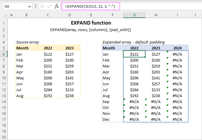
For example, to make the array in C6:D13 expand to 12 rows and 3 columns, use this formula:
=EXPAND(C6:D13, 12, 3)
Because we didn’t set a pad_with value, Excel will fill the extra cells with #N/A.
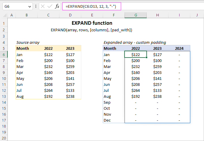
To fill the new cells with a different value, simply add it to the formula. For example, to use a hyphen (-) instead of #N/A, write:
=EXPAND(C6:D13, 12, 3, “-“)
Below you will find a few more examples of using the EXPAND function in Excel to grow an array in a specific direction.
Expand array to a certain number of rows
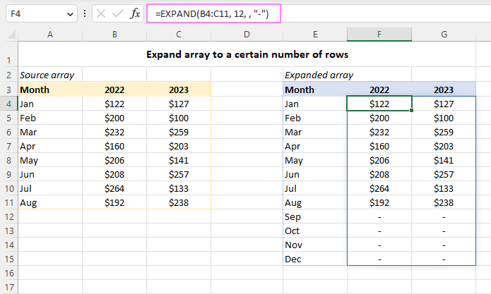
To extend an array to a specific number of rows, you only need to set the rows argument and leave the columns argument blank.
For example, if you want the array from C6:D13 to have a total of 12 rows, use this formula:
Since you don’t want to change the columns, put a comma after the rows argument. Then, after the comma, add the padding value (in this case, a hyphen) for the new cells.
Expand array to a certain number of columns
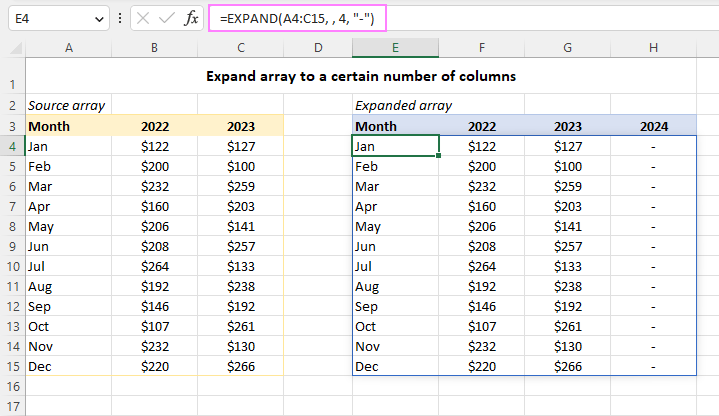
To add extra columns to an array, only specify the columns argument and leave the rows argument empty.
For example, if you want the array in A4:C15 to have a total of 4 columns, use this formula:
Here, leaving the rows argument blank (with a comma) tells Excel to keep the same number of rows while adding columns. The hyphen (“-“) fills the new cells.
How to expand an array left and up
The EXPAND function can only add new cells to the right and below an array. If you need to add cells to the left or above, you’ll have to find another way.
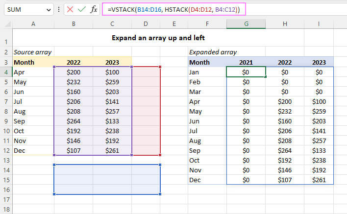
For example, let’s say you have an array in B4:C12, and you want to add 3 rows above and 1 column to the left. To make this easier to understand, we’ll first do each step separately and then combine them into one solution.
Add columns to left
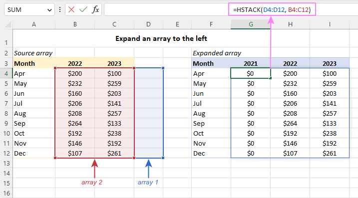
To add extra columns on the left side of an array, you can use the HSTACK function. For example, if you want to add one blank column, use this formula:
Here, the range D4:D12 represents the empty column. Make sure it has the same number of rows as your original array (B4:C12) and that it appears first in the formula. This setup will add a column of zero values to the left of your array.
Add rows above
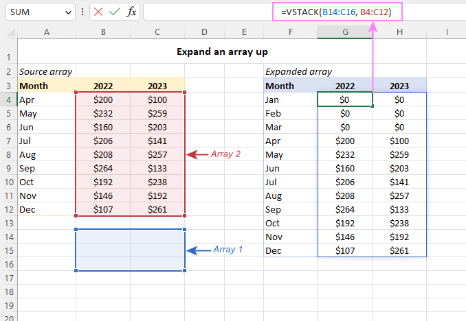
To add extra rows above an array, use the VSTACK function. This stacks new rows on top of your original data.
For example, to add 3 empty rows above the array in B4:C12, use this formula
Here’s how it works:
- B14:C16 is the empty range (it should have the same number of columns as the original array).
- B4:C12 is the original array.
- Since the empty range comes first, Excel adds 3 rows with zero values at the top.
Add rows above and columns to left
To expand an array both up and left, you need to combine VSTACK and HSTACK by placing one inside the other.
In this case, use the formula:
=VSTACK(B14:D16, HSTACK(D4:D12, B4:C12))
Here’s how it works:
- HSTACK(D4:D12, B4:C12) → Adds a blank column to the left of the original array.
- VSTACK(B14:D16, … ) → Adds blank rows above the new expanded array.
This formula increases the array size both vertically and horizontally in one step.
Pad an array up and left with custom value
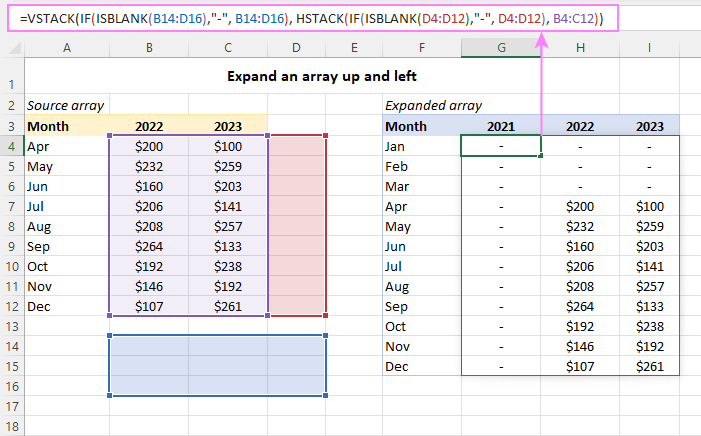
By default, VSTACK and HSTACK fill new cells with zeros instead of leaving them blank. If you want to fill them with a custom value, you can use IF and ISBLANK inside each function. This will replace blank cells with the value you choose.
For example, to fill the new cells with a hyphen (-) instead of zeros, use this formula:
=VSTACK(IF(ISBLANK(B14:D16),”-“, B14:D16), HSTACK(IF(ISBLANK(D4:D12),”-“, D4:D12), B4:C12))
Here’s how it works:
- IF(ISBLANK(B14:D16),”-“, B14:D16) → Replaces blanks in the extra rows with “-“.
- IF(ISBLANK(D4:D12),”-“, D4:D12) → Replaces blanks in the extra column with “-“.
- HSTACK adds the new column to the left.
- VSTACK adds the new rows on top.
This way, all new cells will be filled with hyphens instead of zeros!
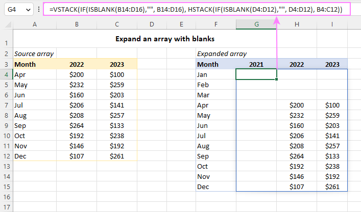
To extend an array with blank cells, use this formula:
=VSTACK(IF(ISBLANK(B14:D16),””, B14:D16), HSTACK(IF(ISBLANK(D4:D12),””, D4:D12), B4:C12))
Split strings and expand arrays
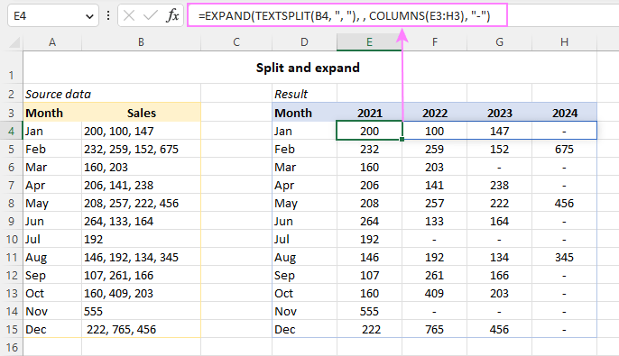
This example shows how to use EXPAND and TEXTSPLIT together to split text into separate columns and make sure all results have the same size.
Imagine you have a list of text strings in column B. Each string contains multiple values separated by a comma and a space (“, “). Your goal is to split these values into separate columns, ensuring that each row has the same number of columns.
To do this, enter the following formula in E4:
=EXPAND(TEXTSPLIT(B4, “, “), , COLUMNS(E3:H3), “-“)
How the formula works:
- TEXTSPLIT(B4, “, “) → Splits the text in B4 into separate values using “, “ as the separator.
- COLUMNS(E3:H3) → Counts the number of columns in the target range to determine how wide the result should be.
- EXPAND(… , , COLUMNS(E3:H3), “-“) → Expands the array to match the required number of columns, filling any missing values with hyphens (“-“).
Finally, drag the formula down through E15, and all the rows will be evenly formatted!
That’s how to use the EXPAND function in Excel to extend an array to as many rows and columns as your business logic requires. I thank you for reading and hope to see you on our blog next week!


