Excel Tables – Complete & Advanced Guide 2025
What is Excel Tables?
Excel tables organize data into rows and columns with special features like unique names for columns, easy-to-use formulas, automatic formatting, and simple sorting and filtering. They make data management and analysis more efficient.
Table of Contents
Download Practice File
Creating Excel Table

- On the Insert tab, in the Tables group, click “Table“
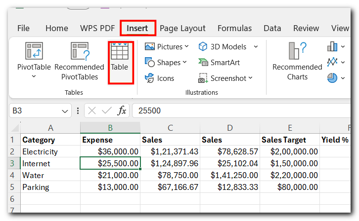
- Excel will automatically select the data range. Make sure to check “My table has headers” and then click OK.
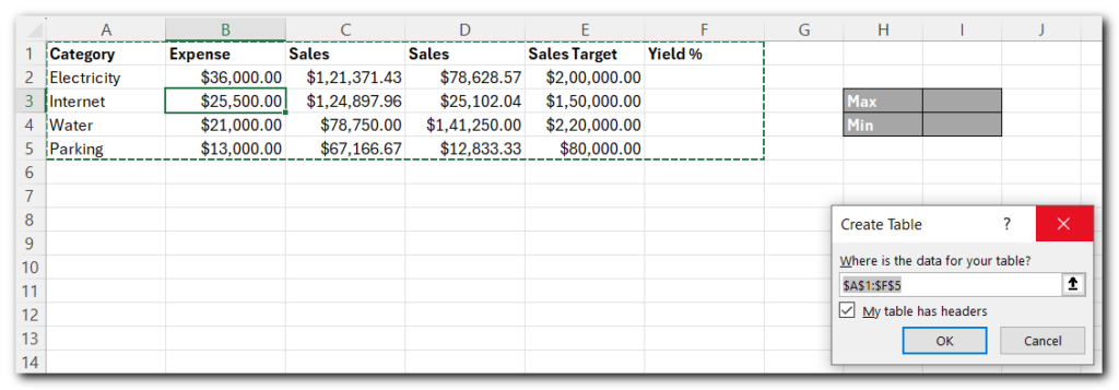
Result: Excel creates a nicely formatted table for you. Although it may look like a regular data range, many powerful features are now just a click away.

Shortcut to Create Excel Tables
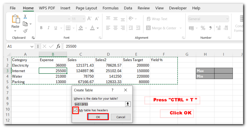
You can quickly create a table in Excel using a shortcut. Here’s how:
1. Select the range of cells you want to include in the table.
2. Press “Ctrl + T” on your keyboard.
3. In the “Create Table” dialog box, ensure the range is correct and check “My table has headers” if your data has headers.
4. Click “OK”.
Your selected range will be converted into a table with formatted rows and columns, and filter buttons added to the headers.
Formatting Excel Tables
Step 1:- Convert Table into Range
Note:-Converting a table to a range in Excel removes table-specific features like filter buttons and structured references. However, your data stays in the same layout.
- Select Table: Click anywhere inside the table.
- Go to the Table Design tab (or Table Tools tab), and click Convert to Range in the “Tools” group. Confirm by clicking Yes.
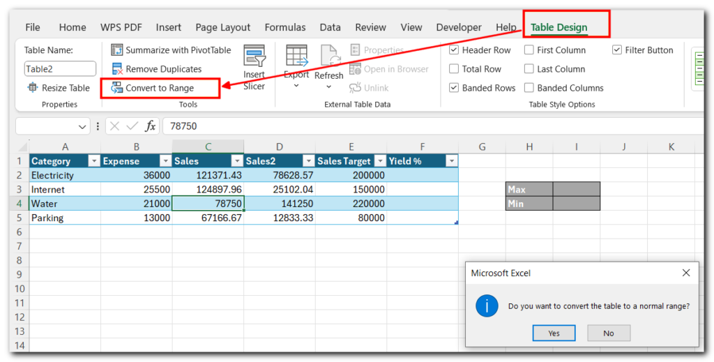
Now, you can format the range as needed.

Step 2:- Clear Previous Formatting:
- Go to the Home tab.
- In the Font group, Font Color select Automatic, click the Fill Color drop-down and select No Fill.
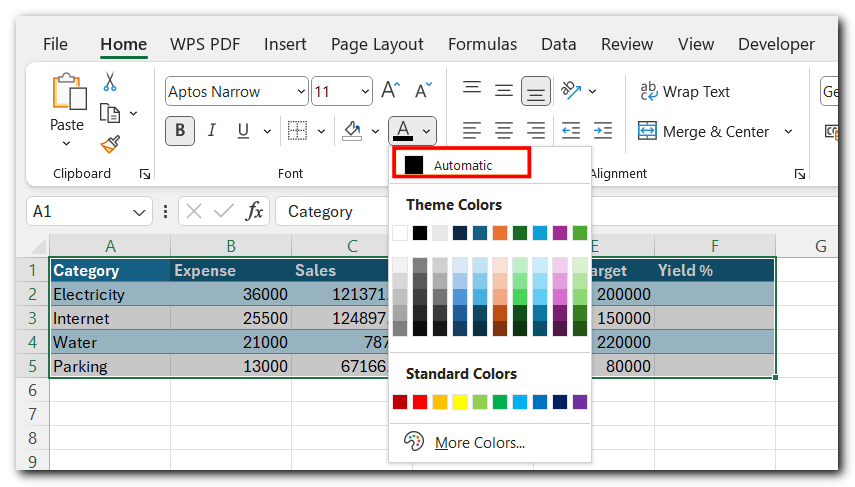
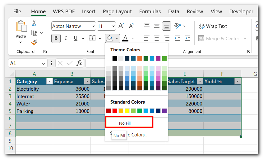
- Click the Borders drop-down and select No Border.
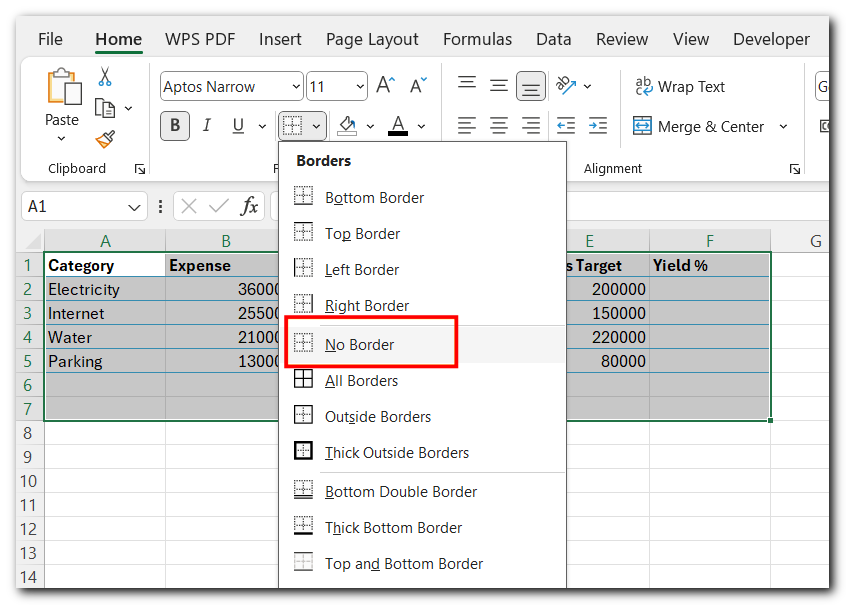
Your data is now free of any previous formatting and ready to be formatted into a table.

Step 3:-Formatting Excel Table
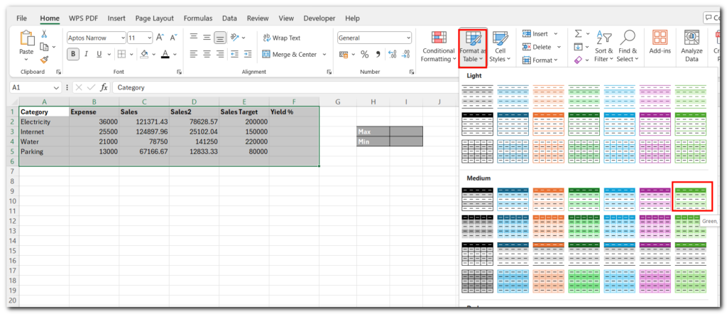
- With your data range selected, go to the Home tab.
- In the “Styles” group, click Format as Table.
- Choose a table style from the gallery.
- Ensure the range is correct and check “My table has headers” if applicable. “Click OK”
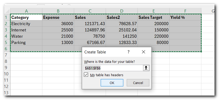
Your data is now formatted as a table with the selected style.

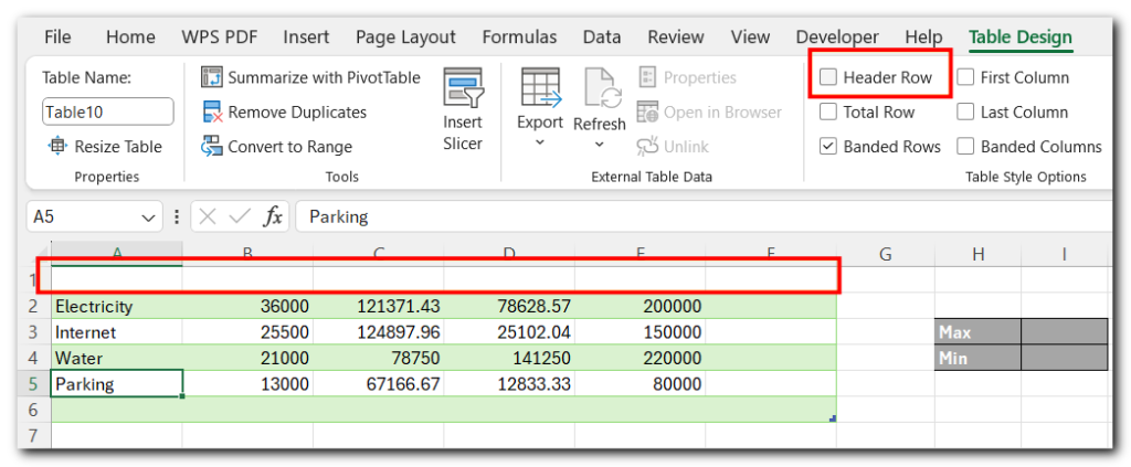
Header Row in Excel Tables
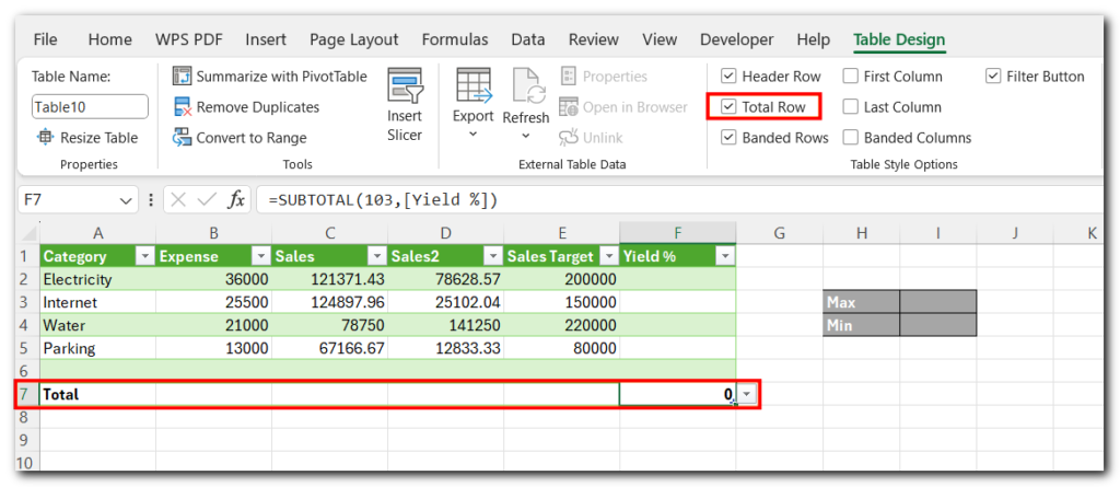
Total Row in Excel Tables
If you check or uncheck the “Total Row” option in Excel table design, it toggles the display of a row at the bottom of the table that shows predefined calculations like sums or counts for selected columns.
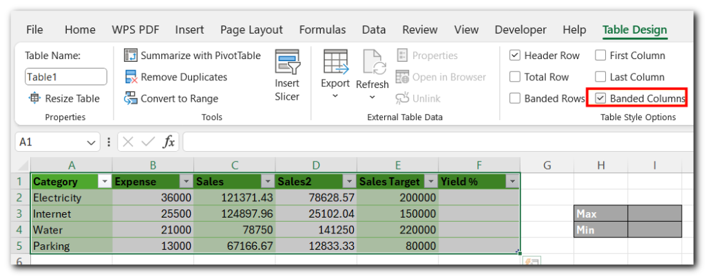
Banded Rows/Columns in Excel Tables
Banded Rows Example:
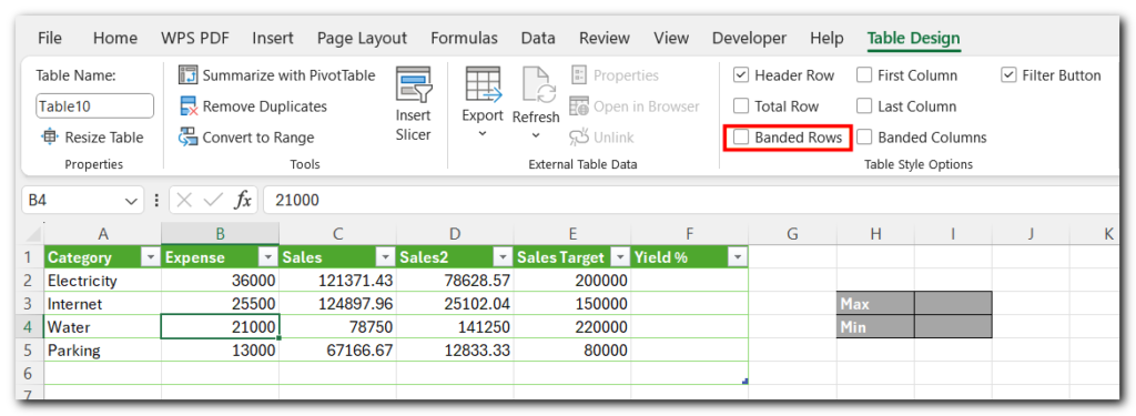
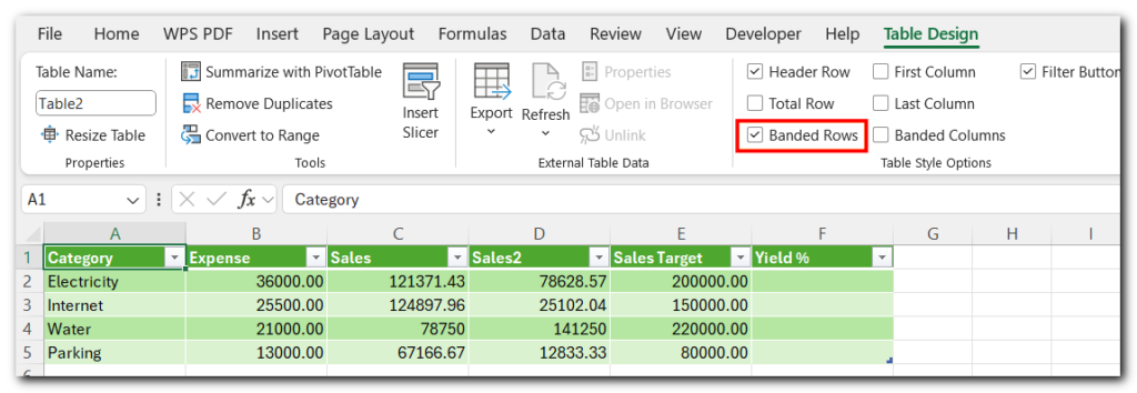
Banded Columns Example:
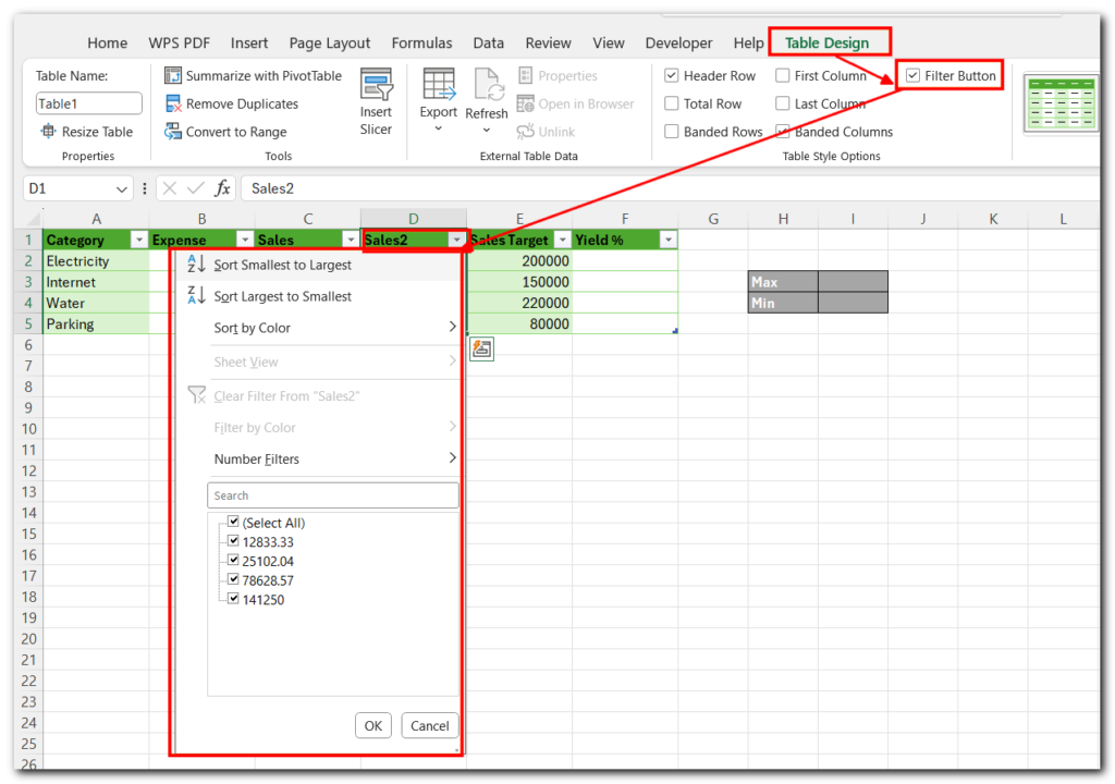
Sorting and Filter in Excel Tables
- Go to the Design tab.
- Ensure the Filter Button is checked.
- Sort and filter toggles will appear in the column headings.
- Click a toggle in any column heading to access the sort and filter menu.
Slicer in Excel Table
- Go to the Design tab in the Table Tools menu.
- Click Insert Slicer.

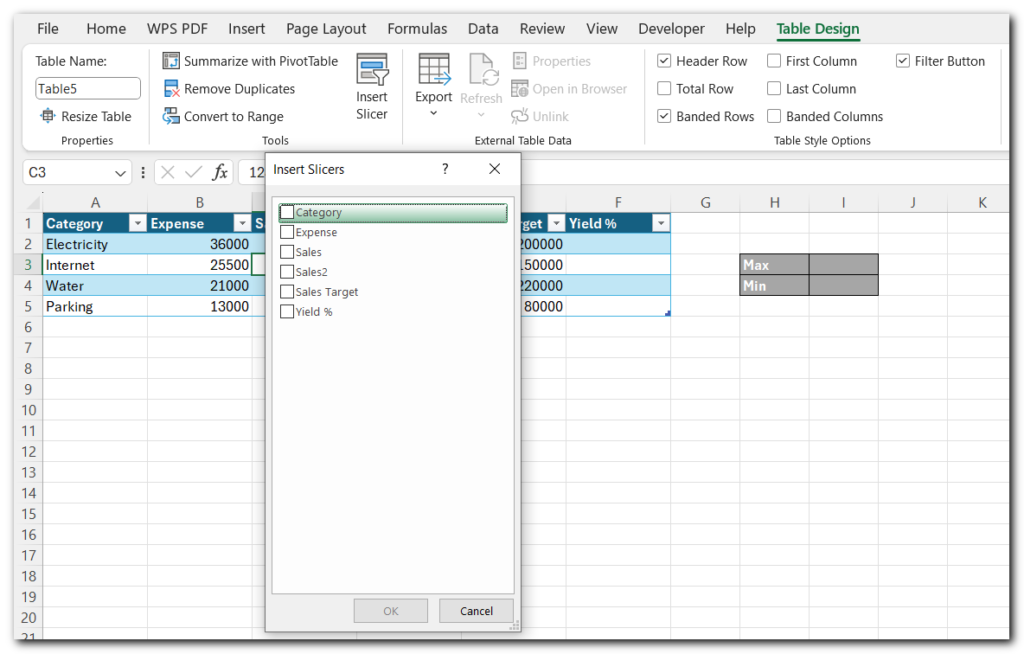
- Check the boxes for the columns you want slicers for (e.g., “Category“.
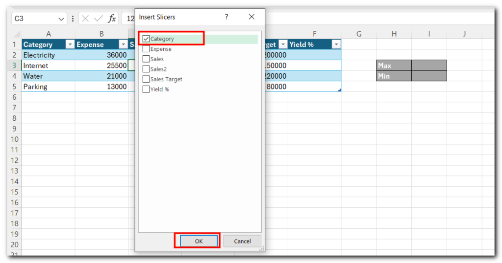
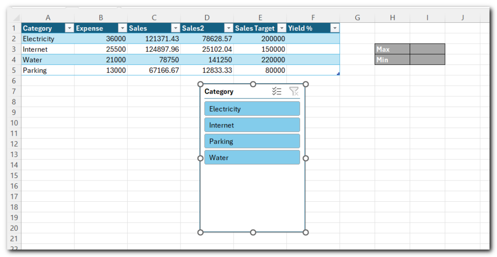
- Click OK: This will add slicers for the selected columns.
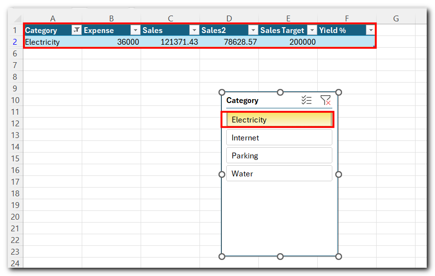
- Click on any button in the slicer to filter the table based on that value. For example, if you click on “Electricity” in a Category slicer, the table will only show rows related to electricity.
This is all “How to add and use slicer in Excel Tables”
Yield% in Excel Tables
Here’s how to calculate yield percentage in Excel:
- Add a new column for “Yield Percentage”
- Enter Formula in cell F2. Use columns “Initial Value” and “Final Value” write formula =(D2/E2) and press “Enter”

You’ll have the yield percentage calculated.

- Select cells in column F2, right-click, choose “Format Cells,” and pick “Percentage.”
- Drag the fill handle from C2 down to apply the formula to other cells.
That’s it! You’ll have the yield percentage calculated for each row.
Conclusion
Excel tables are powerful tools for organizing and analyzing data. However, there are times when you may need to simplify your data. Converting a table to a range can remove unnecessary features while keeping your data intact and easy to work with. This flexibility allows you to choose the best way to manage your data for any situation
Hope you like this article, follow us to learn more about Excel tips.


