SEARCH function is used to find “position of character or text” in an available cell.
Search function is NOT case sensitive, means it will search “r” for text contains “r” and “R”. If you want to find value with case sensitive, then try FIND Function
=SEARCH(find_text,within_text,[start_num])
find_text argument, is the used to give character/ text or cell reference for which position is required to find
within_text argument, is used to give the cell reference from which find_value to be searched
[start_num] is optional argument and is used to specify the character from which search should be started. By default, the first character is 1, however if you want search should be started from 2nd find_text value then it should be position of 2nd find_text value and so on..
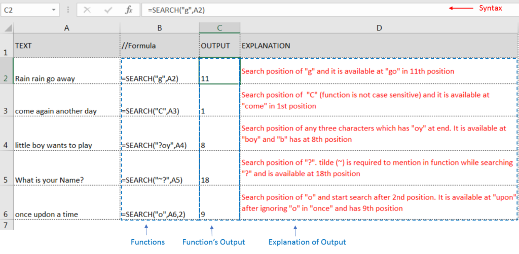
Here we have some examples, where:
– “Column A has various strings,
– “Column B” shows the sample formula that is applied,
– “Column C” shows the output of the function and
– Explanation is provided in Column “D”

– Search function will also work with Wild characters i.e. asterisk (*), question mark (?). Asterisk will find any series of characters and Question mark will find a single character.
– If you want to search actual * or ? (Asterisk or Question Mark) then type tilde (~) before * or ?
– Function should give output in “General” format, however if output is not as per the desired format then we need to change the cell format to “GENERAL”.
– If function parameters are not correctly applied in the function, then it will give output as “#VALUE!”
Don’t forget to leave your valuable comments!
If you liked this article and want to learn more similar tricks, please Subscribe us

Many tasks in Excel require comparing data in different cells. To do this, Excel offers six logical operators, also known as comparison operators. This tutorial will help you understand how these operators work and how to write efficient formulas for data analysis

Microsoft Excel “HOUR, MINUTE, SECOND Functions” are time related functions helps to extract the Hour, Minute or Second from a complete Time.

This tutorial explains how the TRANSPOSE function works and shows you the right way to use it to switch data in Excel.
Everyone has different preferences, even for work habits. Some people like to arrange data in vertical columns, while others prefer horizontal rows. If you ever need to switch the direction of your data quickly, the TRANSPOSE function can help

Watch: How to use WEEKNUM Function in Excel? What is WEEKNUM Function? The WEEKNUM function in Excel returns the week number of a given date. It is a DATE and TIME function that can be…

An easy way to transform an array or range into a column with the TOCOL function. The ability to transpose data from columns to rows and in reverse has been in Excel for quite a…

In this tutorial, we will explore the CHOOSEROWS function in Excel 365 and how to use it in real life. Imagine you have a big Excel sheet with hundreds of rows, and you need to…