Match function is as same as what it means. Match function helps to match the partial or full user defined value or number in a given range and return the exact or relevant position of the same.
For Example: If we have an array i.e. 1,2,3,4 and if I ask you what is the position of 3 in this array, your answer will be 3rd position in the array. We will explain more examples in details.
The MATCH formula uses the following arguments:
Match_type (optional argument) – Match function will helps you to find the location of the lookup value it could be horizontal or it can be vertical. But when you mention horizontal than its horizontal if you mention vertical than its vertical.
Let’s look at few examples here to learn more about Excel Function Match
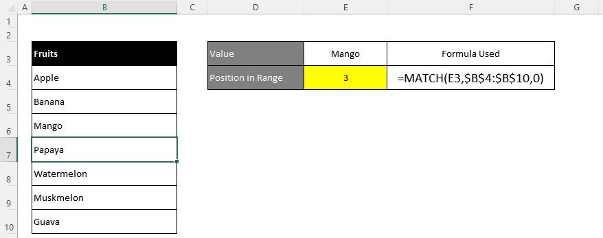
Now here we have range “B4:B10” where all fruits are listed. Now on the right side, we have value in E3 cell “Mango” and we want to get the position of Mango in Fruits data given.

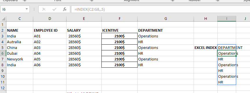
Excel INDEX function is used when you want to pull out the ARRAY RANGE WITH HELP OF formula you can either pull the cell value or you can pull all the AARAY range values with the help of INDEX function.
The formula =INDEX(C2:G8,,5).
In this formula first argument we are selecting


Microsoft Excel “TODAY” function is used to get the current Date. It is very useful function and can be used in many ways. “TODAY Function” does not have any argument that makes this easy to apply and implement.

RANK function performs the Ranking in a range or list of numbers. Function returns the rank position and can assigned as highest or lowest value as 1st Rank

You must have faced a condition when your data cells contain extra spaces, leading spaces or trailing spaces and you wanted to remove these extra spaces to standardize the data. So here you may use…

Watch: How to use SUMIF & SUMIFS Function in Excel? What is SUMIF Function? The SUMIF function in Excel adds up values in a range of cells that meet certain criteria. Click here to Read Full…

SUMIFS function is used to get the “total sum” of values for matching criteria across range. SUMIFS Function has required and optional arguments

In this tutorial, we’re going to explore one of the most intriguing features in Excel: the OFFSET function.
So, what is the OFFSET function in Excel? Simply put, OFFSET gives you a reference to a range of cells that’s moved from a starting point by a certain number of rows and columns.