We can place multiple criteria or conditions in function by separating them with comma ( , )
=COUNTIFS(criteria_range1, criteria1, [criteria_range2, criteria2]…)
criteria_range1 argument is used to give the range in which criteria1 needs to find
criteria1 argument is used to give criteria for count. We can give value (example “A”, >10, 50) or cell reference# (example: F2) in this argument
[criteria_range2] optional argument is used to give the ANOTHER range in which criteria2 needs to find
[criteria2] optional argument is used to give criteria2 for count. Value or cell reference# can be given.
Kindly note, we can add multiple criteria in the function by separating them with Comma ( , )
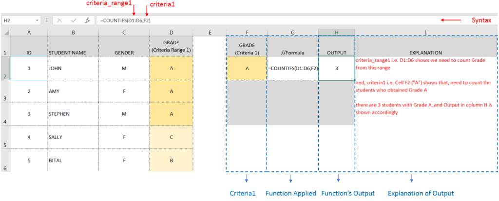
Here, we want to get the count of students who obtained Grade A:
We will be using COUNTIFS function as follows:

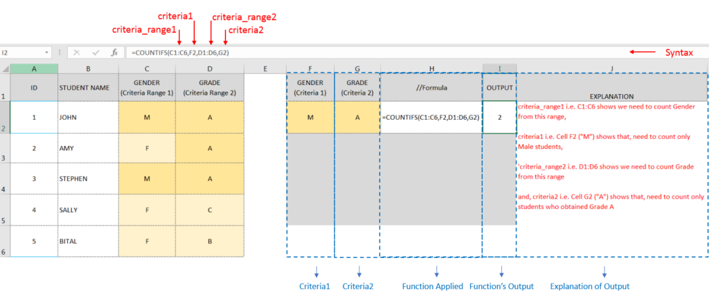
Here, we want to get the count of Male Students (criteria1) who have obtained Grade A (criteria2):
We will be using COUNTIFS function as follows:

Hope you learnt this Function,
Don’t forget to leave your valuable comments!

This tutorial explains how the TRANSPOSE function works and shows you the right way to use it to switch data in Excel.
Everyone has different preferences, even for work habits. Some people like to arrange data in vertical columns, while others prefer horizontal rows. If you ever need to switch the direction of your data quickly, the TRANSPOSE function can help

Watch: How to use VLOOKUP Function in Excel? What is VLOOKUP Function? The VLOOKUP function in Excel searches for a value in a table and returns a corresponding value from another column in the same row…

How to use Excel Function PROPER? PROPER function is used for changing the format of any text or string to PROPER or SENTENCE Case. PROPER Function has argument only one argument i.e. text, which makes the function…
This tutorial explains the idea of “SPILL Range” in easy-to-understand language and answers common questions. Spilling is a new feature in Excel 365 that comes with dynamic arrays. To use it well, it helps to…

SUMIF function is used to get the “total sum” for number of times the criteria across range is met. SUMIF Function has two required arguments.

This tutorial explains how to use the IFERROR function in Excel to catch and handle errors. It shows you how to replace errors with a blank cell, a different value, or a custom message. You’ll also learn how to use IFERROR with functions like VLOOKUP and INDEX MATCH, and how it compares to other error-checking functions like IF ISERROR and IFNA