We can place multiple criteria or conditions in function by separating them with comma ( , )
=COUNTIFS(criteria_range1, criteria1, [criteria_range2, criteria2]…)
criteria_range1 argument is used to give the range in which criteria1 needs to find
criteria1 argument is used to give criteria for count. We can give value (example “A”, >10, 50) or cell reference# (example: F2) in this argument
[criteria_range2] optional argument is used to give the ANOTHER range in which criteria2 needs to find
[criteria2] optional argument is used to give criteria2 for count. Value or cell reference# can be given.
Kindly note, we can add multiple criteria in the function by separating them with Comma ( , )
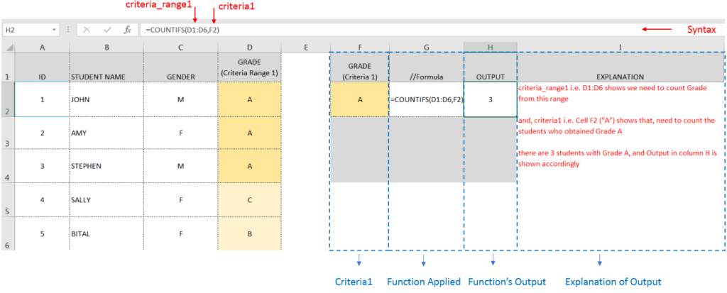
Here, we want to get the count of students who obtained Grade A:
We will be using COUNTIFS function as follows:

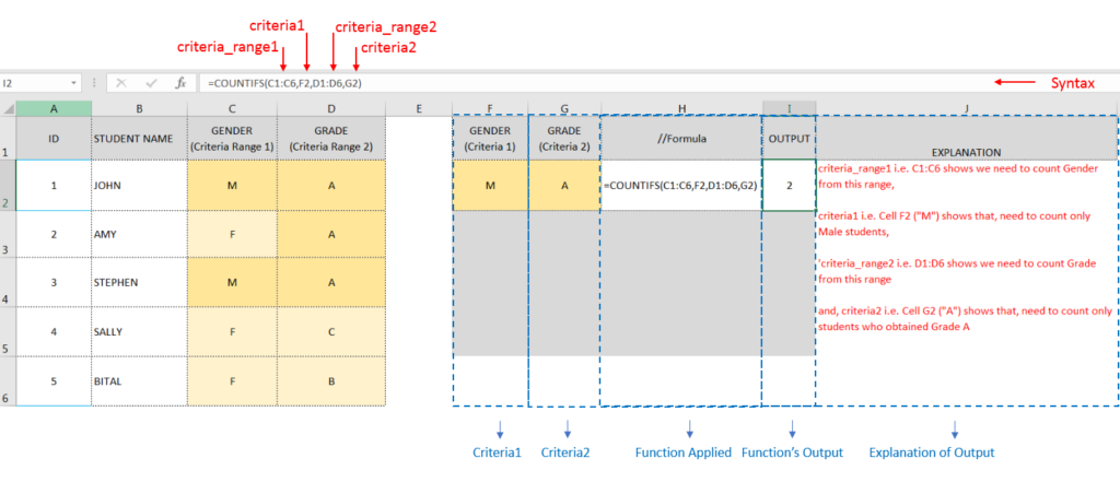
Here, we want to get the count of Male Students (criteria1) who have obtained Grade A (criteria2):
We will be using COUNTIFS function as follows:

Hope you learnt this Function,
Don’t forget to leave your valuable comments!

This guide shows how to use the nested IF function in Excel to check several conditions. You will also learn about other functions that can be to use than a nested formula.
When you want to make decisions in Excel, you often use an IF formula. It checks if something is true, then gives one result if it is and another result if it isn’t. If you need to check more than one thing, you can put many IFs inside each other.
Although using multiple IFs is common, it’s not the only way to check several conditions in Excel. This guide will introduce you to some easier and useful alternatives.

SUBSTITUTE function is used to substitute the existing old text to new text.

Microsoft Excel “DAY, MONTH, YEAR Functions” are date related functions helps to extract the Day, Month or Year from a Date.

This tutorial explains how the TRANSPOSE function works and shows you the right way to use it to switch data in Excel.
Everyone has different preferences, even for work habits. Some people like to arrange data in vertical columns, while others prefer horizontal rows. If you ever need to switch the direction of your data quickly, the TRANSPOSE function can help

RANK function performs the Ranking in a range or list of numbers. Function returns the rank position and can assigned as highest or lowest value as 1st Rank

This tutorial introduces XLOOKUP, a new function in Excel for both vertical and horizontal lookups. Tasks that used to feel super complicated, like left-side lookups, finding the last match, or using VLOOKUP with multiple criteria, are now much easier with XLOOKUP.
Before, you had to choose between VLOOKUP for vertical lookups, HLOOKUP for horizontal ones, or more complex options like INDEX MATCH or Power Query. But now, you don’t have to pick anymore. XLOOKUP can handle all those tasks in one simple function.