=SUBSTITUTE(text,old_text,new_text,[instance_num])
Text argument [Required] is used to give the cell reference in which value to be searched
old_text argument [Required], is used to give the specific text or cell reference, to be substituted
new_text argument [Required], is used to give the specific text or cell reference that you want to substitute in old_text
instance_num argument [Optional], is used to give the occurrence number that you want to substitute
Here we have an example, where “Column A” has various values and are required to substitute year “2018” with “2019”. Output of the function returns value in ”Column B” and explanation is also provided.
We will be following SUBSTITUTE function as follows:
– text argument value “A2” shows the cell reference in which “2018” is to be searched
– old_text argument value “2018” shows that “2018” should be replaced in “A2” cell
– new_text argument value “2019” shows the substituted value
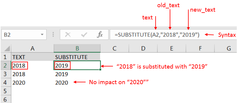
– Value in cell “B2” shows that “2018” in cell “A2” is substituted with “2019”
– Value in cell “B4” shows that cell “A2” did not have “2018” that is why text is not substituted and function returns original value of cell “A2” as output
Here we have another example, where “2018” should be replaced with “2019” but ONLY SECOND OCCCURRENCE. Output of the function returns value in ”Column B” and explanation is also provided.
We will be following SUBSTITUTE function as follows:
– text argument value “A2” shows the cell reference from which “2018” is to be searched
– old_text argument value “2018” shows that “2018” should be searched in “A2” cell
– new_text argument value “2019” shows the substituted value
– instance_num argument value “2” shows only 2nd occurrence to be substituted and there should no impact on other values.
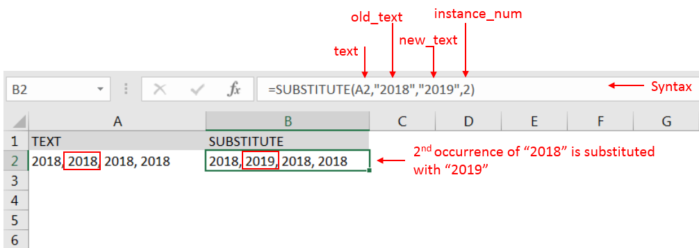
– Value in cell “B2” shows that “2018” in cell “A2” is substituted with “2019” but only 2nd occurrence and there is no impact on
– Spaces available in a string is counted as characters
-Value in instance_num argument should NOT be negative
– If value in old_text argument is not searched in text argument cell, function will return value of text argument cell
– If cell reference or parameters are not correctly provided in the function, then it will give output as “#VALUE!” (Error).
– Function should give output in “General” format, however if output is not as per the desired format then we need to change the cell format to “GENERAL”.
Hope you learnt this Function,
Don’t forget to leave your valuable comments!
If you liked this article and want to learn more similar tricks, please Subscribe us or follow us on Social Media by clicking below buttons:
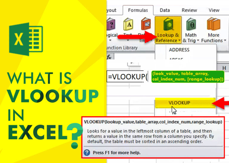
An ultimate guide for basic user to understand Excel Vlookup function. VLOOKUP is a vertical lookup which helps the user to extract the values from other columns (leftmost) basis on matching column string.
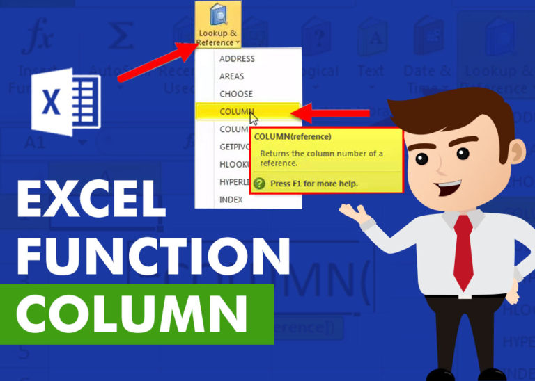
COLUMN function is used to get the column reference number of the excel worksheet. COLUMN Function has only one argument.

AND, OR, NOT Functions” provide result in “TRUE” or “FALSE”. If the logical condition is correct and matching the parameters provided, then result would be “TRUE” or if logical condition is not correct and not matching the parameters provided then result would be “FALSE”
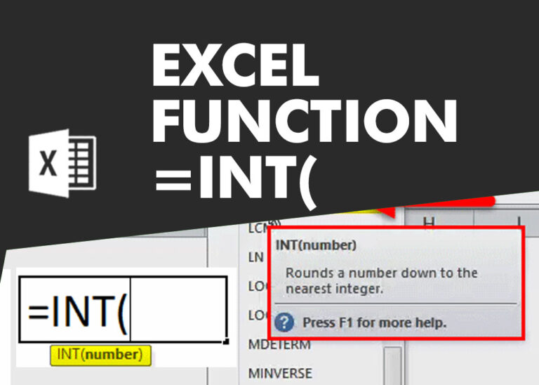
INT function is used to round down the numeric value to nearest integer. INT Function has one required argument i.e. number.

Microsoft Excel “TODAY” function is used to get the current Date. It is very useful function and can be used in many ways. “TODAY Function” does not have any argument that makes this easy to apply and implement.

What is COUNTIFS in Excel? The Microsoft Excel COUNTIFS function counts the number of cells in a range, that meets a single or multiple criteria and adjacent or non-adjacent. As a Statistical function of Excel,…