How to Calculate Weighted Average in Excel?
Microsoft Excel is a useful tool for analyzing data and conducting statistical research. The program includes numerous functions for performing various statistical calculations. One of the essential measures Excel supports is the weighted average.
In this article, we’ll guide you through the steps to calculate weighted averages in Excel using both the SUM and SUMPRODUCT functions. Additionally, we’ll share tips to help you make the most of these features.
The weighted average of a dataset calculates the average based on the importance of each value in the sample. When you compute the weighted average, you multiply each value by its assigned weight before finding the average. This method helps in analyzing statistical functions such as correlations and probabilities.
When dealing with smaller samples, calculating the weighted average is straightforward. For instance, a teacher might use the weighted average to assess exam scores. As data becomes more complex, using Excel to calculate weighted averages can simplify the process.
Weighted Average formula
First things first, what is a weighted average?
You will understand this by looking at the weighted average formula.
Here’s some data for when you go grocery shopping.
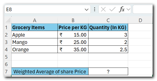
The grocery list includes apples, mangoes, and oranges, each with different prices per kg.
So, what is the weighted average price per kg for all these items?
We buy different quantities of each item. To find the weighted average, we need to multiply each item by its weight.
This means multiplying the price of each grocery item by the quantity bough
- Write the formula as follows
= SUM (B2*C2, B3*C3, B4*C4)
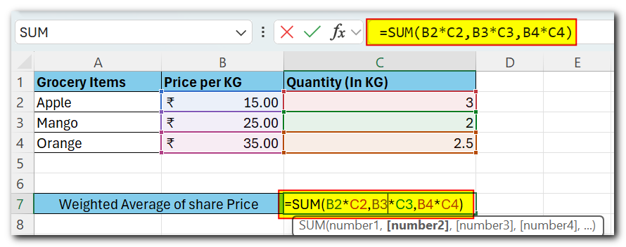
The results are as follows
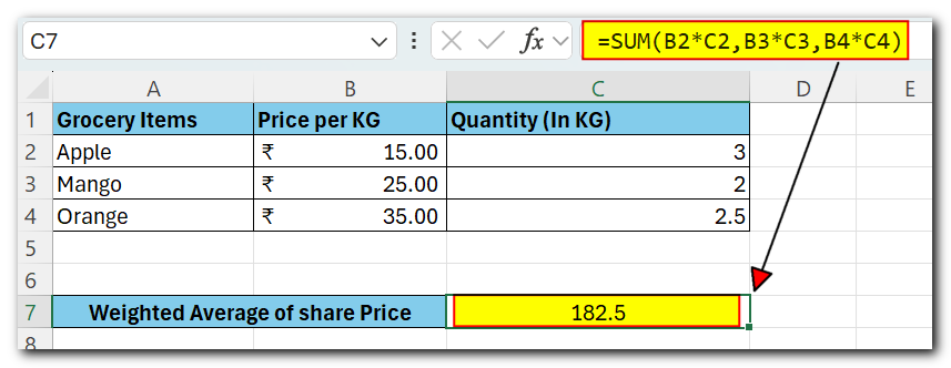
Here, we multiplied the price of each grocery item by its quantity. Then, we added all these values together
- Divide the total from the previous step by the sum of all the quantities of the grocery items.
= SUM (B2*C2, B3*C3, B4*C4) / SUM (C2:C4)
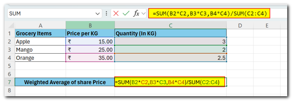
Here are the results.
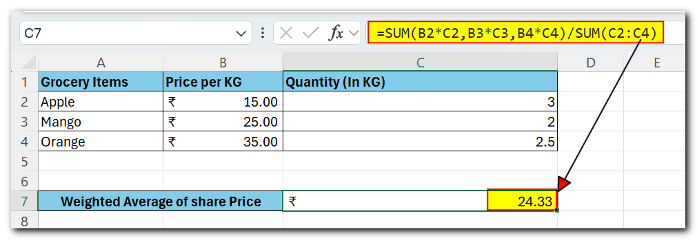
The $24.33 shows the weighted average price of all the grocery items.
Difference between Weighted Average vs Normal Average
How is the weighted average different from the normal average? Why do we even need it?
Here’s the answer.
The image below shows data for shares of three companies.
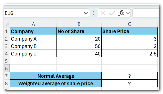
The data above shows the portfolio of an investor. It includes both the number of shares and their prices.
What is the average share price of the portfolio?
Simply use the average function as shown below.
- Write the AVERAGE function as =AVERAGE (C12:C14)
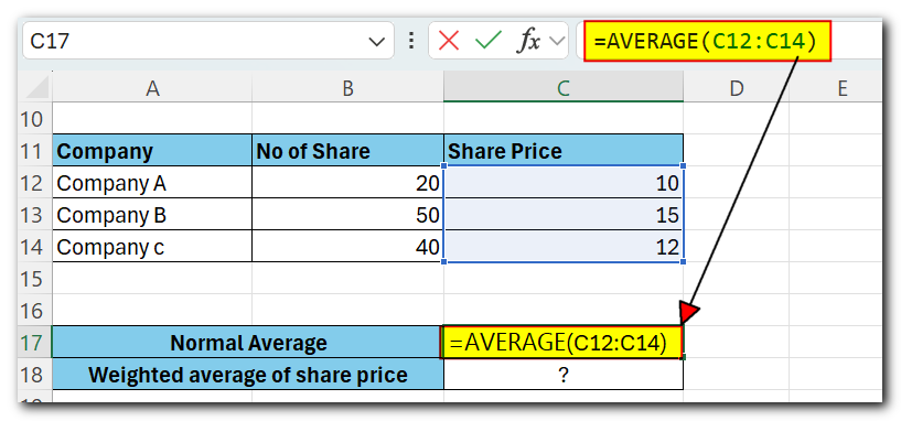
- This results in a simple average of these three share prices.
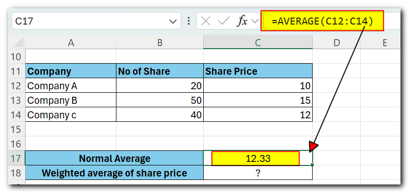
But does this number accurately represent the average share price for this portfolio?
No, because we have a different number of shares for each company. Therefore the weight of each share price is different.
- To calculate the weighted average share price, create a new column
- Write the following formula to multiply the number of shares of each by the share price
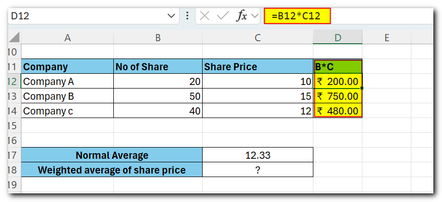
- Calculate the sum of the number of shares and the above column
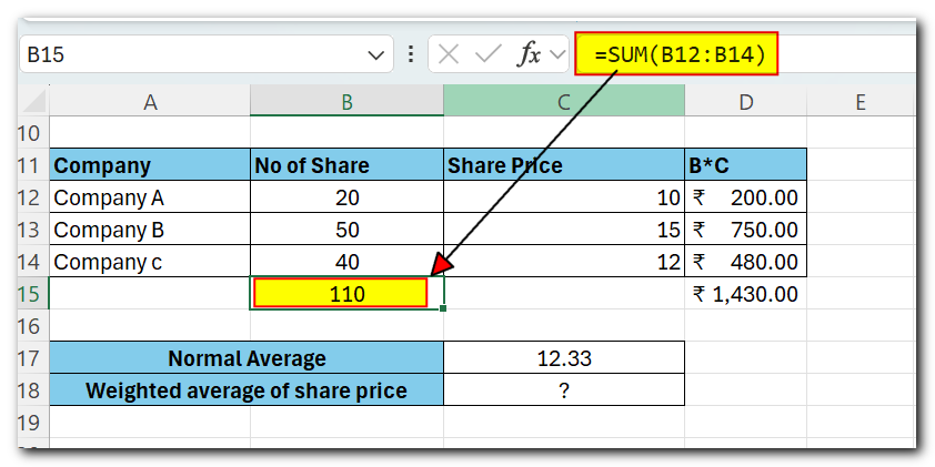
- Calculate the average as follows.
= D15 / B15
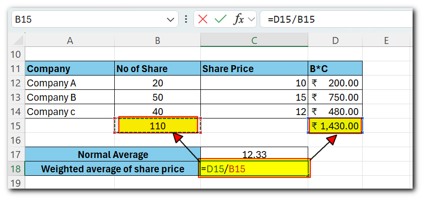
D15 contains the sum of the share prices multiplied by the number of shares. B15 contains the total number of shares.
- The weighted average comes as follows.
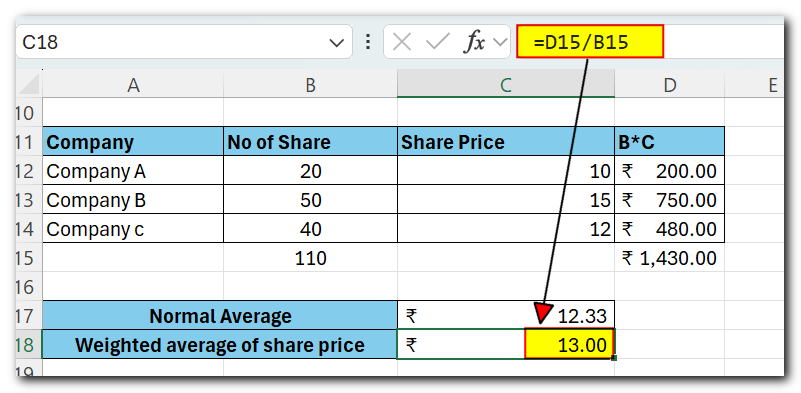
The answer changes a lot, from $12.33 to 13.00.
This is how the weighted average differs from the normal average. It doesn’t just divide the sum of values by the number of values.
It multiplies each share price by the number of shares, then divides the total by the total number of shares.
With data like this, the weighted average is much more accurate than the normal average.
Weighted average with SUMPRODUCT function
Excel doesn’t have a built-in function for calculating weighted averages.
However, the closest function to do this in Excel is the SUMPRODUCT function.
Let’s use the same example as above. To find the weighted average of the share prices, follow these steps.
Write the SUMPRODUCT function below.
= SUMPRODUCT (B23:B25, C23:C25)
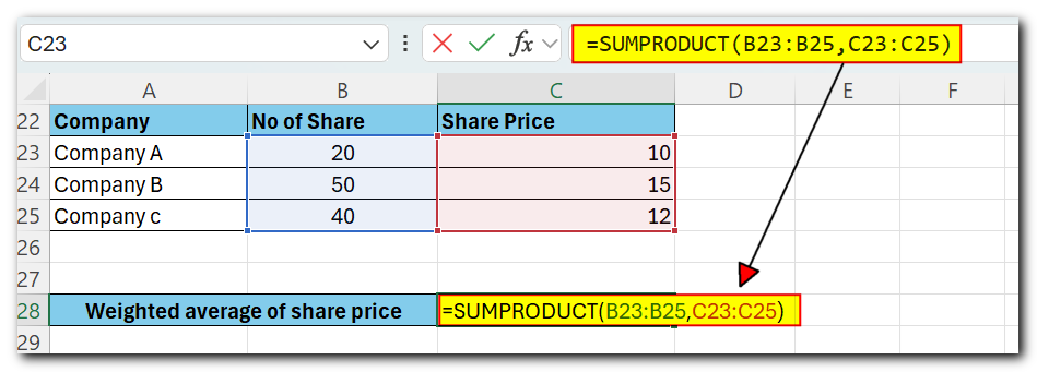
What does this function do? It adds up the cells in the ranges B23:B25 and C23:C25.
Next, it multiplies these sums. That’s why it’s called the SUMPRODUCT function. It sums the values in two ranges and then multiplies the results
- Here is the result of the SUMPRODUCT function.
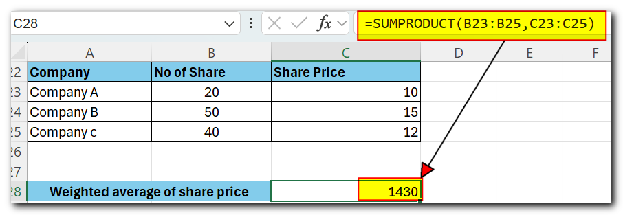
- Next, we need to divide it by the total number of shares
- To the above SUMPRODUCT function, add the SUM function as below

This divides the sum of the result of the SUMPRODUCT function by the SUM of the shares
- The weighted average comes out as follows

Although Excel doesn’t have a built-in function specifically for calculating weighted averages, there are several ways to achieve this in Excel.
In the article above, we learned how to set up a formula to calculate weighted averages in Excel. We also discussed the differences between weighted average and normal average, and how their results differ.
Finally, one effective method to calculate the weighted average in Excel is by combining two functions: SUMPRODUCT and SUM
 New Excel VBA Course Live Now! $49 for first 100 Students Only


