TEXTSPLIT function in Excel: split cells text by delimiter
This tutorial explains how to use the new TEXTSPLIT function in Excel 365 to break text into separate parts using any symbol or space you choose.
Sometimes, you may need to split text in Excel. In older versions, we could do this using tools like Text to Columns and Flash Fill. Now, Excel 365 has a special function called TEXTSPLIT, which makes it even easier. This function lets you split text into different columns or rows based on the rules you set.
Table of Contents
Excel TEXTSPLIT function
The TEXTSPLIT function in Excel helps you break text into separate parts using a chosen symbol or space. It can split the text into different columns, rows, or both. The result appears automatically in multiple cells.
This function has six options, but you only need to use the first two for it to work.
Text (Required) – The text you want to split. You can type the text directly or use a cell reference.
Col_delimiter (Required) – The symbol or character that tells Excel where to split the text into columns. If this is left out, you must use Row_delimiter instead.
Row_delimiter (Optional) – The symbol or character that tells Excel where to split the text into rows.
Ignore_empty (Optional) – Decides what to do with empty values:
- FALSE (default) – Creates empty cells when there are two or more separators in a row.
- TRUE – Skips empty values, so no extra empty cells appear.
Match_mode (Optional) – Decides if the delimiter should be case-sensitive:
- 0 (default) – Case-sensitive (treats uppercase and lowercase as different).
- 1 – Case-insensitive (treats uppercase and lowercase as the same).
Pad_with (Optional) – A value to fill missing spaces when splitting text in two directions (both columns and rows). If not set, Excel shows #N/A error for missing values.
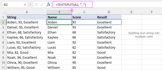
For example, to divide a text string in A2 into multiple cells using a comma and a space as the separator, the formula is:
=TEXTSPLIT(A2, “, “)
TEXTSPLIT availability
The TEXTSPLIT function is only available in Excel for Microsoft 365 (Windows and Mac) and Excel for the web.
Basic TEXTSPLIT formula to split a cell in Excel
For starters, let’s see how to use a TEXTSPLIT formula in its simplest form to split a text string by a particular delimiter.
Split a cell horizontally across columns
To break the contents of a cell into several columns, you first provide the cell reference containing the text and then give the delimiter (the character where you want to split the text).
For example, to split the text in cell A2 at each comma, use this formula:
=TEXTSPLIT(A2, “,”)
Here, the delimiter is a comma inside double quotes (“,”). This means each piece of text separated by a comma will appear in its own column.

Remember, you only need to enter the formula in one cell (for example, C2). The results will automatically spread into the nearby cells.
The group of cells filled by the formula is called a spill range. Excel highlights this area with a blue border, showing that all the values inside come from the formula in the top-left cell.
Split text by substring
Often, the values in your text are separated by more than one character. For example, a comma followed by a space (“, “) is common. To handle this, simply use the full string (“, “) as your delimiter.
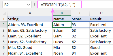
For example, to split the text in A2 into separate columns using a comma and a space, use this formula:
=TEXTSPLIT(A2, “, “)
Enter this formula in B2 and then copy it down to fill as many cells as needed.
Split string into columns and rows at once
To split text into both rows and columns at the same time, you need to set both delimiters in your TEXTSPLIT formula.
For example, if you want to break the text in cell A2 into rows and columns, use:
- An equal sign “=” as the col_delimiter.
- A comma and a space “, ” as the row_delimiter.
The complete formula looks like this:
=TEXTSPLIT(A2, “=”, “, “)
This formula returns a 2-D array with 2 columns and 3 rows.

Separate cells by multiple delimiters
If your text has different or inconsistent separators, you can use an array constant {…} for the delimiter. This allows Excel to recognize multiple delimiters at once.
For example, if the text in A2 is separated by commas (“,”) and semicolons (“;”), with or without spaces, you can use this formula to split it into rows:
=TEXTSPLIT(A2, , {“,”,”, “,”;”,”; “})
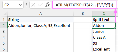
Alternatively, if you only want to split by commas and semicolons, but also remove extra spaces, use the TRIM function:
=TRIM(TEXTSPLIT(A2, , {“,”,”;”}))
This keeps your data clean by removing unwanted spaces.
Split text ignoring empty values
If your text has two or more consecutive delimiters without anything between them, you can decide whether to ignore the empty spaces or not. This is controlled by the ignore_empty parameter, which is set to FALSE by default.
By default, TEXTSPLIT does not ignore empty values, and this works well for data that is organized in a structured way.
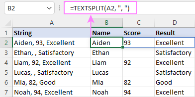
For example, in the table below, some scores are missing. If you use the TEXTSPLIT formula without the ignore_empty argument, or set it to FALSE, Excel will create an empty cell for each missing value:
=TEXTSPLIT(A2, “, “)
Or
=TEXTSPLIT(A2, “, “, FALSE)
This way, all the values, including the empty ones, will appear in the correct columns.
In case your strings contain homogeneous data, it may stand to reason to ignore empty values. For this, set the ignore_empty argument to TRUE or 1.
For instance, to divide t the below strings placing each skill in a separate cell without gaps, the formula is:
=TEXTSPLIT(A2, “, “, ,TRUE)
In this case, the missing values between consecutive delimiters are ignored completely:

Cell splitting case-sensitive or case-insensitive
You can decide whether TEXTSPLIT should treat uppercase and lowercase letters as the same by using the match_mode argument (the fifth option in the formula).
By default, match_mode is 0, which makes TEXTSPLIT case-sensitive. This means it will only recognize the delimiter exactly as you type it.
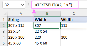
For example, if numbers are separated by both lowercase “x” and uppercase “X”, the following formula will only split by lowercase “x”:
=TEXTSPLIT(A2, ” x “)
Important: The delimiter ” x ” includes spaces on both sides. This helps remove extra spaces from the results.
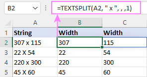
To turn off case sensitivity, you supply 1 for match_mode to force the TEXTSPLIT formula to ignore the letter case:
=TEXTSPLIT(A2, ” x “, , ,1)
Now, all the strings are split correctly by either delimiter:
Pad missing values in 2D array
The last option in the TEXTSPLIT function, called pad_with, is useful when some values are missing in the text.
When splitting a string into both columns and rows, Excel usually shows #N/A errors in place of missing values. This helps keep the table structure correct.
For example, in the text below, there is no “=” sign (col_delimiter) after the word “Score”. Because of this, TEXTSPLIT fills the missing space with #N/A to keep the data properly aligned.

To make the result more user-friendly, you can replace the #N/A error with any value you want. Simply, type the desired value in the pad_with argument.
In our case, that could be a hyphen (“-“):
=TEXTSPLIT(A2, “=”, “, “, , ,”-“)

Or an empty string (“”):
=TEXTSPLIT(A2, “=”, “, “, , ,””)

Now that you’ve learned practical uses of each argument of the TEXTSPLIT function, let’s discuss a couple of advanced examples that can help you cope with non-trivial challenges in your Excel spreadsheets.
Split dates into day, month and year
To split a date into individual parts (like month, day, and year), you first need to convert the date into text. This is because the TEXTSPLIT function only works with text, while Excel dates are stored as numbers.
The easiest way to turn a number into text is by using the TEXT function. Just make sure to use the right format for your date.
For example, to convert a date in A2 to text, use this formula:
=TEXT(A2, “m/d/yyyy”)
Next, put this formula inside the TEXTSPLIT function as the first argument. Then, choose the delimiter (like a slash “/”) for the second argument, depending on whether you’re splitting across columns or rows.
Since the date units are separated by slashes, the final formula looks like this:
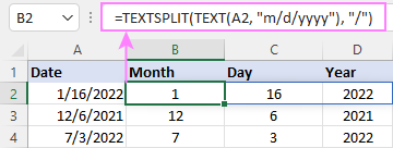
=TEXTSPLIT(TEXT(A2, “m/d/yyyy”), “/”)
This will split the date into separate parts: month, day, and year.
Split strings skipping certain values
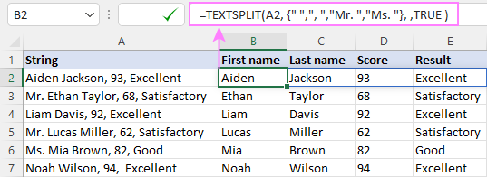
Supposing you want to separate the below strings into 4 columns: First name, Last name, Score, and Result. The problem is that some strings contain the title “Mr.” or “Ms.”, because of which the results are all wrong:

The trick might not be obvious, but it’s actually very simple! 😊
Along with the usual space (” “) and comma with space (“, “) as delimiters, you also add “Mr. “ and “Ms. “ to the list of delimiters. This way, TEXTSPLIT uses these titles to split the text correctly.
To make sure there are no extra empty cells, you set ignore_empty to TRUE.
Here’s the formula:
=TEXTSPLIT(A2, {” “,”, “,”Mr. “,”Ms. “}, ,TRUE)
Now, the results are perfectly organized! 🎉
TEXTSPLIT alternatives
In older Excel versions that do not support TEXTSPLIT, you can still split text by combining functions like SEARCH or FIND with LEFT, RIGHT, and MID. Here’s how:
- SEARCH (case-insensitive) or FIND (case-sensitive) finds where the delimiter is in the text.
- LEFT, RIGHT, and MID then extract the part of the text before, after, or between the delimiters.
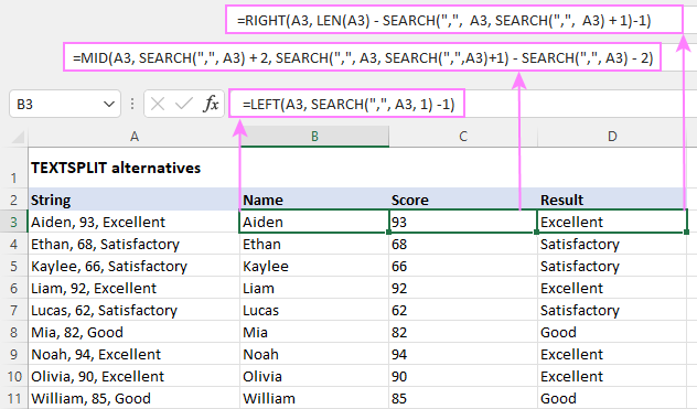
For example, if the values in cell A2 are separated by a comma and a space, you can use these formulas:
- To extract the name:
- =LEFT(A2, SEARCH(“,”, A2, 1) – 1)
- To pull the score:
- =MID(A2, SEARCH(“,”, A2) + 2, SEARCH(“,”, A2, SEARCH(“,”, A2) + 1) – SEARCH(“,”, A2) – 2)
- To get the result:
- =RIGHT(A2, LEN(A2) – SEARCH(“,”, A2, SEARCH(“,”, A2) + 1) – 1)
For a detailed explanation of these formulas, see the guide “How to split strings by character or mask.”
Remember, unlike the dynamic array TEXTSPLIT function, these formulas must be entered separately in each cell. You put the formula in the first cell and then drag it down to apply it to the cells below.
The screenshot below shows the results.
And that’s how you can split cells in Excel 365 using TEXTSPLIT or other methods for older versions!
Thank you for reading! 😊 I hope this guide was helpful, and I look forward to seeing you on our blog next week! 🚀


