How to Split Cells in Excel?
Download Practice File
Microsoft Excel helps you organize and work with data in many ways. When you have a lot of information or need to break it into parts, splitting cells is very useful. Split cells in Excel means taking the content of one cell and dividing it into multiple cells. This can be especially helpful for separating names, addresses, or other data that are combined in one cell. Learn how to split cells in Excel using its built-in functions and formulas.
Splitting cells in Excel is very easy. If you have many values in one cell and want to spread them out across multiple cells, Microsoft Excel offers simple options to do this. This guide will show you the techniques and methods to split cells in Excel, helping you manage and organize your data better for analysis and presentation.
Table of Contents
How to Split Cell using text to columns?
The easiest way to split cells is by using the Text to Columns function. Let’s see how to split a cell diagonally in Excel.
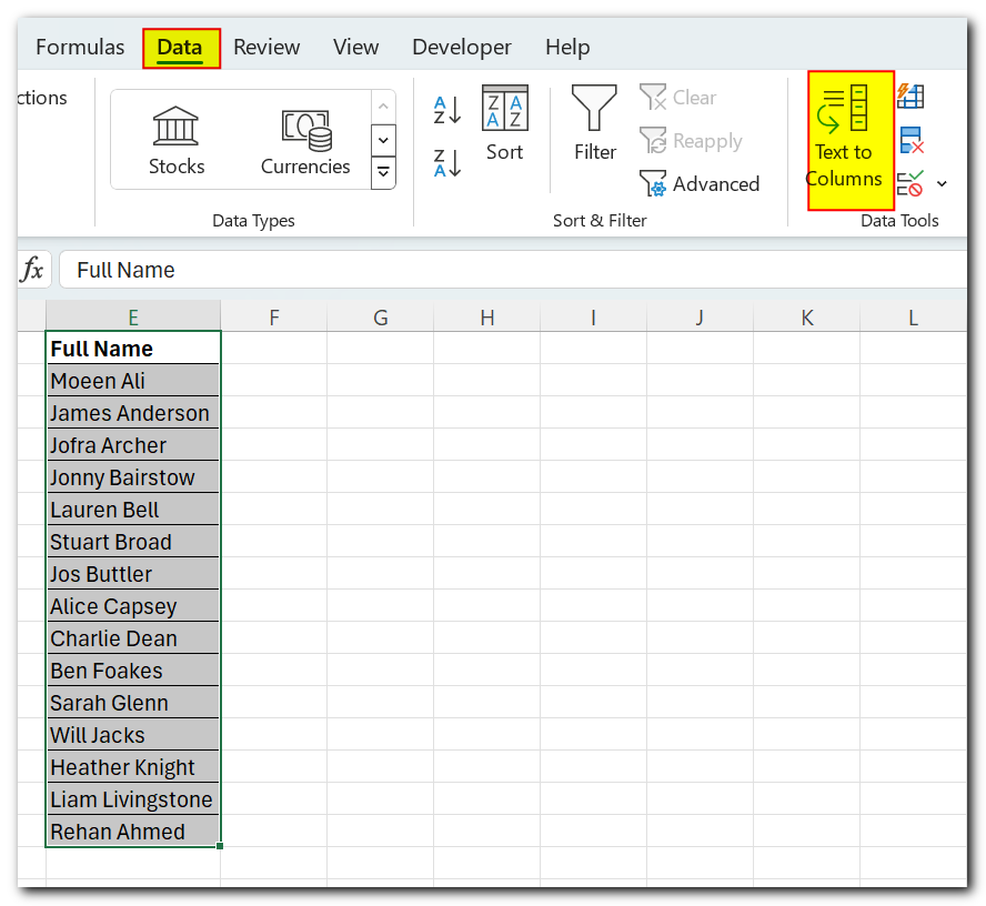
Here are some names that we need to split into two parts
Select all the cells that you want to split.
Locate Data ⇒ Data Tools ⇒ Text to Columns
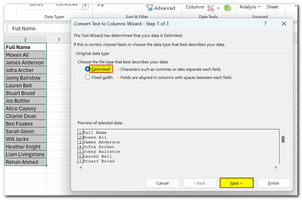
A Convert Text to Columns wizard will appear. Select the file type that matches your data. For this example, we will choose “Delimited.”
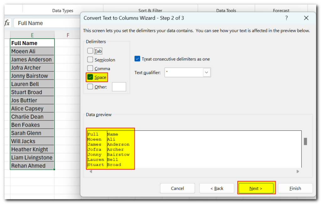
In the next step, we will choose the delimiter for our data. Since the names are separated by spaces, we will select “Space.” If your data uses a different delimiter, choose the appropriate option. In the data preview, you can see how the cell will be split.
Press “Next” to set the data format. Choose “General” if you don’t need any advanced settings.
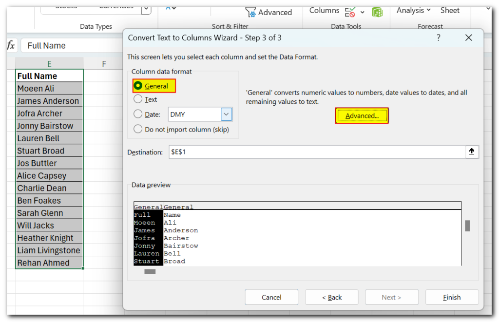
You can choose “Advanced Settings” if you are working with numbers and want to recognize numeric data.
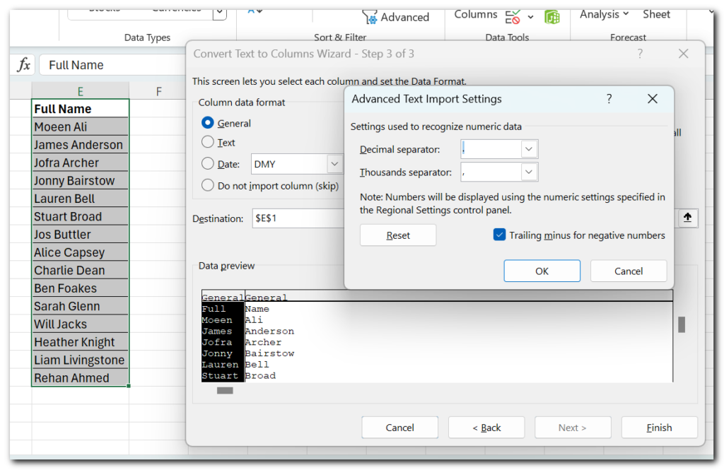
Since we don’t need any extra settings, we will click “Cancel” and then “Finish” after selecting “General.”
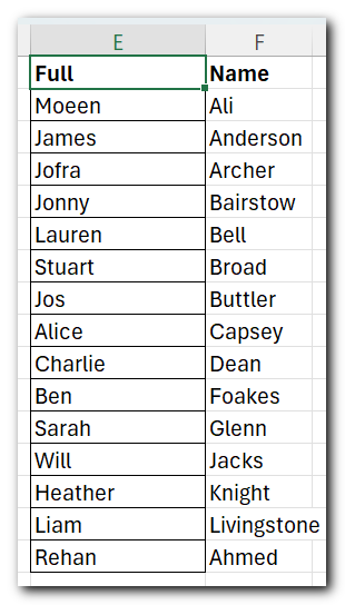
The cell has now split into 2.
Split Cells Diagonally
We have already seen how to split a cell and its contents in Excel. Next, we will show you how to split an Excel cell diagonally. Don’t worry, it’s easy. Just follow these steps:
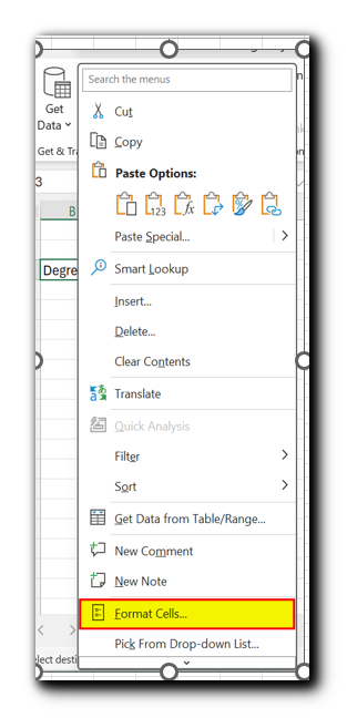
- Select the cell you want to split diagonally, right-click, and choose the “Format Cells” option, as shown in the image below.
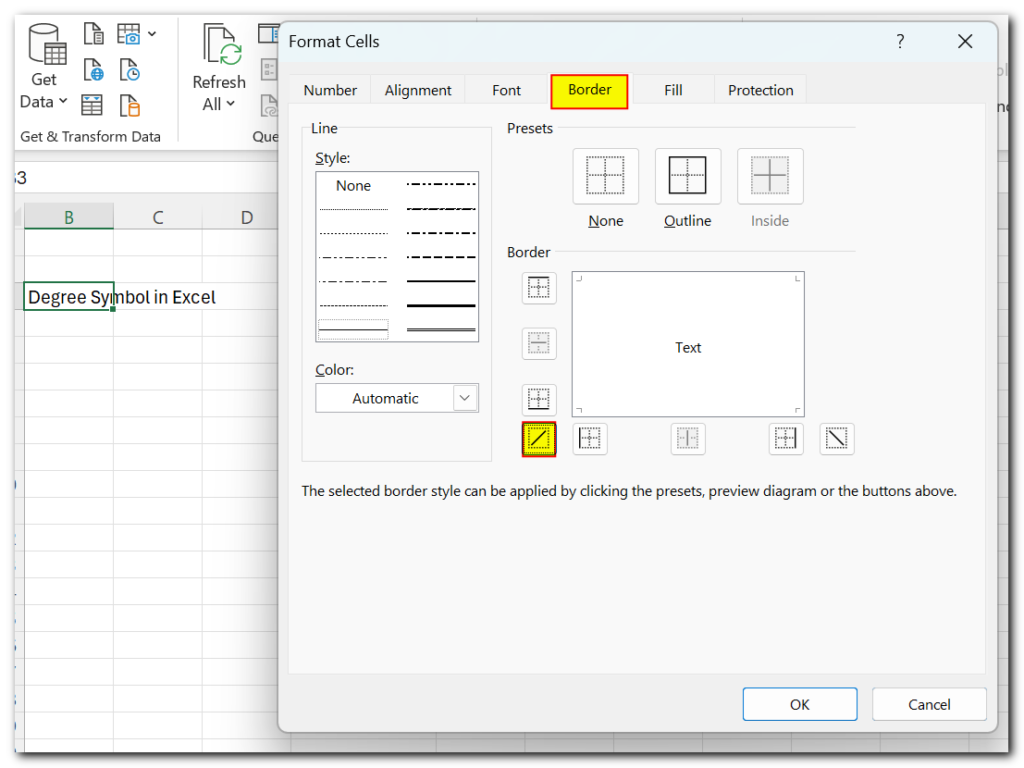
- In the dialogue box, go to the Border tab and click the button containing the diagonal artwork, and then click OK.
Once you’ve clicked OK, we’ll have our cell divided diagonally
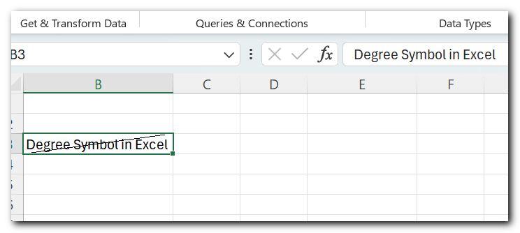
Next, highlight the first word and go to the Fonts tab located in the Home tab’s bottom corner of the Fonts group
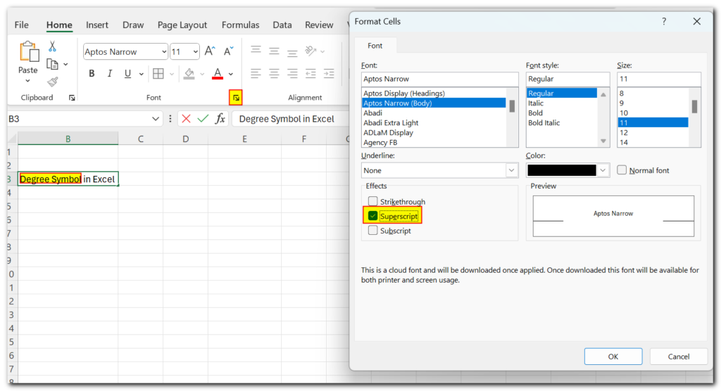
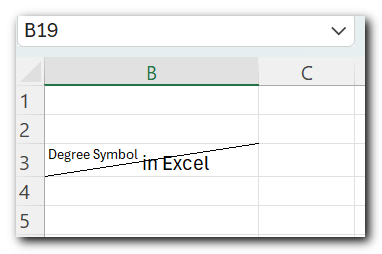
In the dialogue box, check the Superscript box and click OK. Then, repeat the same procedure for the other word, but you will put the Subscript option on this one and click OK.
Lorem ipsum dolor sit amet, consectetur adipiscing elit. Ut elit tellus, luctus nec ullamcorper mattis, pulvinar dapibus leo.
Flash Fill for Splitting cells
You should know about this commonly used Excel function. You need to tell Excel how you want your data to split using Flash Fill.
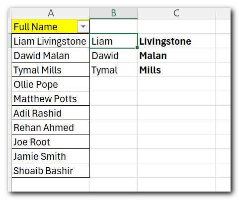
We will go to –
Data ⇒ Data Tools ⇒ Flash Fill
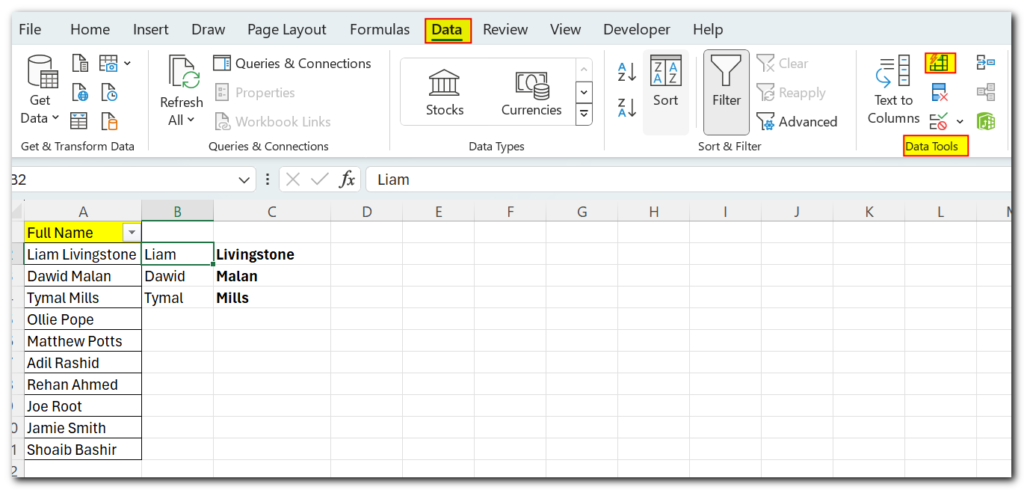
Now, follow the same process for the next part of the string.
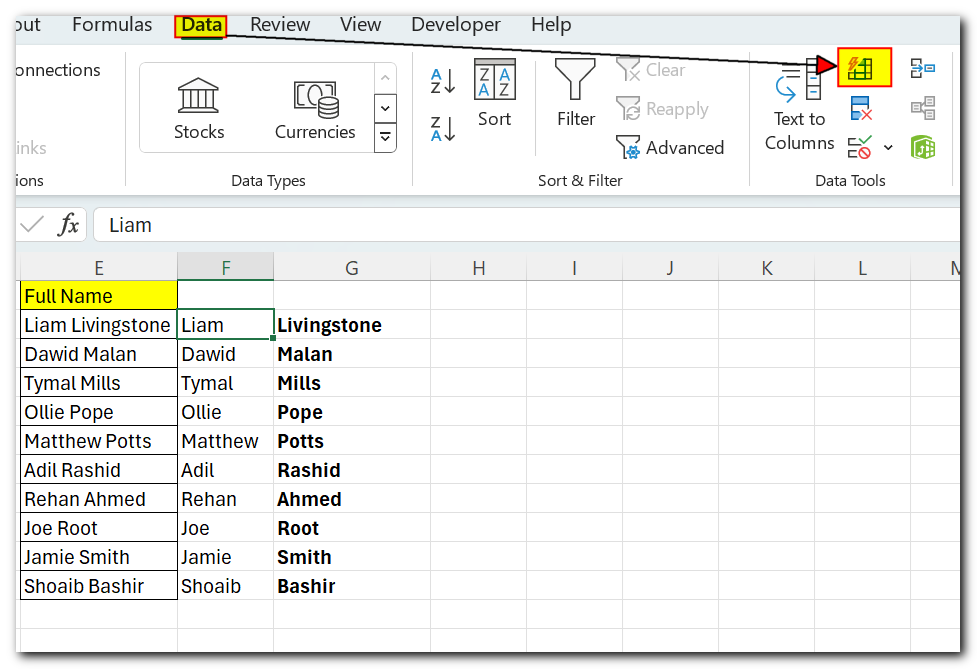
Excel Text Function for Splitting Cells
You can split a cell in Excel using different text functions. These functions help you extract parts of a cell to move to another cell.
Text functions in Excel include:
– Left() – Extracts characters from the left side of text
– Right() – Extracts characters from the right side of text
– Mid() – Extracts characters from the middle of text
– Find() – Locates a substring within another string
– Len() – Returns the total number of characters in a text string
You don’t need all these functions just to split cells, but you can use them in formulas to get the results you need.
For example, you can extract the name using the Left and Find functions. The Find function is helpful because it tells you where the delimiter character, like a space, is located.
Here’s how the function would look:
=LEFT(A2,FIND(” “,A2))
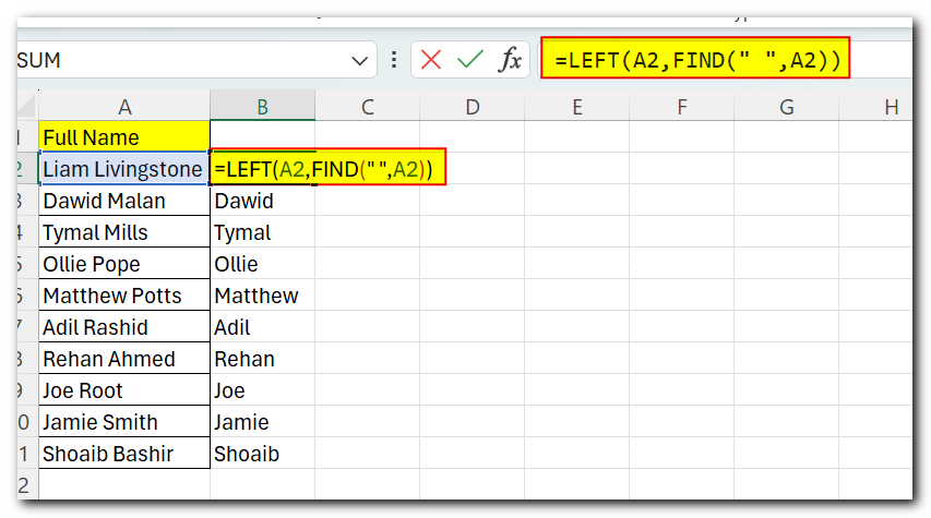
When you press enter after typing this formula, you will see that the first name is extracted from the string in cell A2
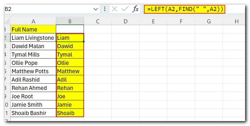
This works because the Left function requires the number of characters to extract. By using the Find function to locate the space character, you can determine the number of characters needed to extract the name.
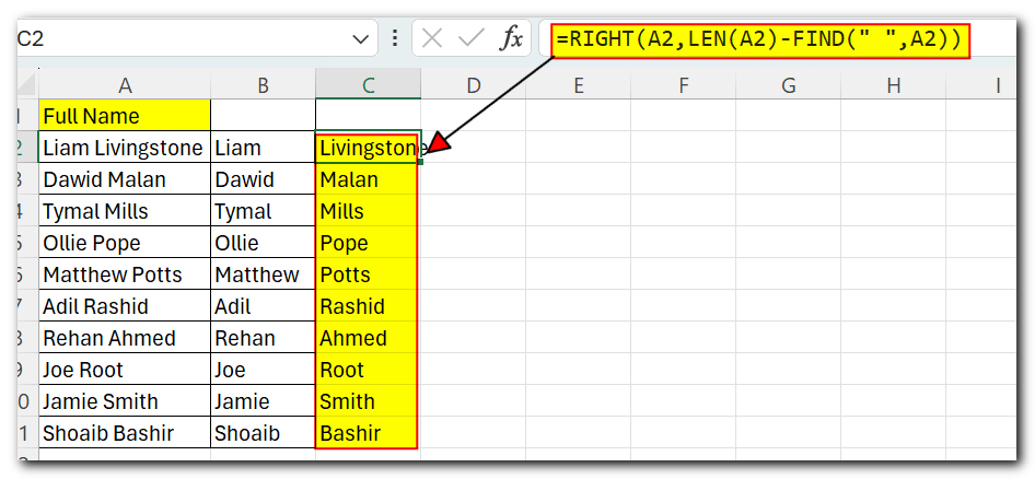
To extract the last name using the Right function:
=RIGHT(A2,LEN(A2)-FIND(” “,A2))
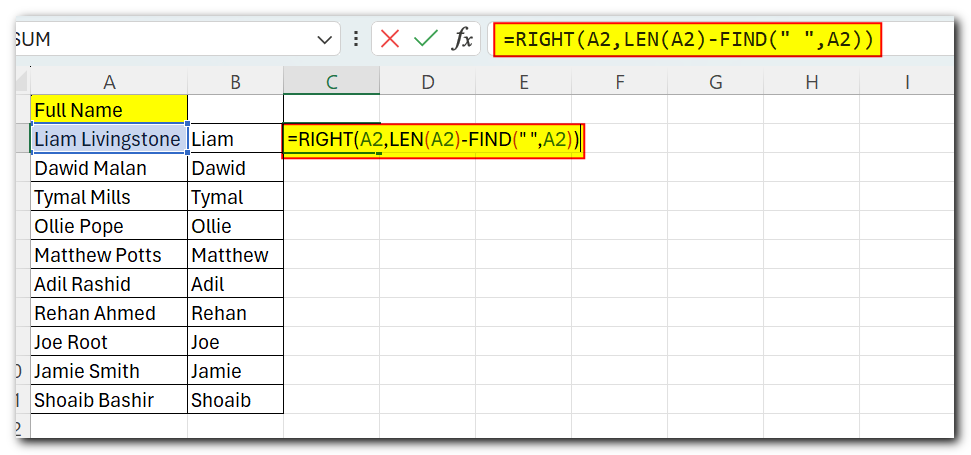
This will extract the last name by finding the position of the space and subtracting it from the total string length. This provides the Right function with the number of characters it needs to extract the last name.
Splitting cells in Excel is a versatile way to organize your data and make it easier to read. You can structure your Excel sheet effectively by using Text to Columns, formulas, or Flash Fill. Mastering these techniques will save you time and make your work more accurate. Remember to think about your data and what you want to achieve when deciding how to split cells.
I hope this article has been helpful to you.


