Excel spill range explained
This tutorial explains the idea of “SPILL Range” in easy-to-understand language and answers common questions.
Spilling is a new feature in Excel 365 that comes with dynamic arrays. To use it well, it helps to understand some basic terms. This will make it easier to follow examples and create your own dynamic array formulas. The main goal of this tutorial is to help you understand what a spill range is and how it works.
Table of Contents
Spill range in Excel
When a dynamic array formula gives more than one result, it automatically spills those values into nearby cells on the worksheet.
The group of cells filled by the formula is called the spill range. It shows all the values returned by the formula.
If you click on any cell in the spilled area, Excel highlights the whole group with a blue border. This means all the values inside the border come from the formula in the top cell.
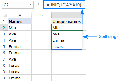
In the past, with older array formulas (called CSE formulas), you had to guess how many cells to select before entering the formula. Now, with dynamic arrays, you just type the formula in one cell, and Excel fills in the rest for you.
The spill range adjusts itself automatically. If your source data changes — like when you add or remove items — the spilled range will grow or shrink to match.
If you delete the formula in the first (top) cell, all the spilled results will disappear.
Spill range reference (# operator)
To refer to a whole spill range, put a hash tag (#) after the address of the upper left cell in the range (i.e. the cell containing the formula that returns an array of values). In terms of Excel, this is called a spill range reference.
For example, we have a UNIQUE formula in C2, which returns multiple results. To reference all those values, type:
=C2#
To refer to the same spill range from another sheet, include the sheet’s name followed by the exclamation point:
=Sheet1!C2#
To reference the spill range from another workbook, also include the file’s name enclosed in square brackets:
=[Book1.xlsx]Sheet1!$C2#
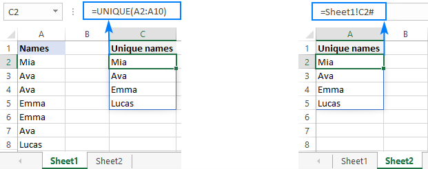
Using C2# in a formula is the same as using a regular range like C2:C5. But the # (spill reference) is smarter — it automatically updates if the number of values changes. So, if your data grows or shrinks, you don’t have to fix your formulas by hand.
This is super helpful when you’re using the spill range in another function — whether it’s a dynamic one or a regular one. You can also use spill references for named ranges or data validation, like when creating a dropdown list that updates on its own.
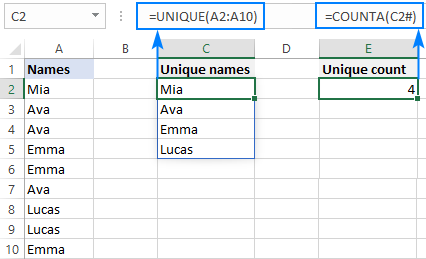
For example, if you want to count how many unique names the dynamic array in C2 returns, just use this formula:
=COUNTA(C2#)
It will always count the right number of names, even if the list changes.
3 things you should know about Excel spill range
The spill range is a great feature that makes working in Excel much easier. Here are a few interesting things to know about how it works:
Only the top-left cell can be edited
The formula lives only in the top cell of the spilled area. That’s the only cell you can edit. If you click on any other cell in the blue-outlined area, you’ll still see the formula in the formula bar — but it will be greyed out, meaning you can’t change it from there.
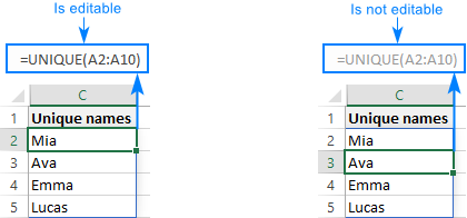
When you change the formula in the first cell and press Enter, Excel automatically updates all other values in the spilled area.
What is and what is not included in spill range
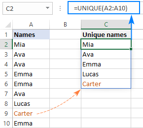
As mentioned above, the spilling behavior is dynamic – when the original data changes, the spilled area adjusts accordingly. For example, if you change the original list so that it contains one more unique name (Carter), the spill range automatically expands to include that name.
However, the spill range does not update when new entries are added outside the referred range.
For example, if the formula refers to A2:A10, and a new item is entered in A11, it won’t appear in the results:
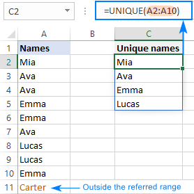
To include a new item in the formula results, you need to update the range from A2:A10 to A2:A11.
But if you want Excel to update the results automatically when new data is added, it’s better to use an Excel table. Just turn your source data into a table and use structured references in your formulas. Excel tables grow on their own when you add new rows, so you don’t have to update the range yourself.
You can also get the same automatic update by using a dynamic named range.
#SPILL error
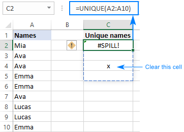
If something is blocking the spill range — like other data, empty spaces, hidden characters, or formulas in the cells below — you’ll get a #SPILL! error.
To fix it, just clear the cells that are in the way.
For more help, check out: SPILL error in Excel – causes and fixes.
How do you clear spill range in Excel?
Depending on what you want to do, there are two easy solutions:
- If you’re getting a #SPILL! error because the spill range isn’t empty, you can either:
- Clear the data that’s blocking the spill area, or
- Move the formula to another spot where there’s enough empty space for all the results.
(For more details, check the link above.)
- If you want to remove all the values in the spill area, just delete the formula in the first (top-left) cell.
How do you change spill range in Excel?
As the spill range is the result of a formula, it cannot be changed manually.
In case you need to modify or update the formula, select the upper left cell in the spilled area, make the required changes and press the Enter key.
How do you fix a spill range if it's too big?
The size of a spill range is decided by Excel and it automatically changes when your source data or formula is updated.
In some cases, you can control the size of the spill range from inside the formula. For example, you can limit how many rows are returned by a formula like FILTER. (See: How to limit the number of rows returned by FILTER.)
If you ever see a #SPILL! error, take a look at this guide: How to fix a #SPILL! error in Excel.
How do you get rid of spill range in Excel?
The answer depends on what you want to do:
- Disable spilling completely:
You cannot turn off spilling for all of Excel. There is no setting for that because spilling is a very useful feature. It’s better to learn how to work with it. - Remove a spill range:
To remove a spill range, just delete the formula in its first cell. - Stop a formula from spilling into many cells:
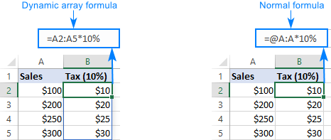
Use the @ symbol to restrict the formula to one value. This is called implicit intersection.
For example, if you use this formula:
=A2:A5*10%
Excel multiplies each value in A2:A5 by 10%, and the result spills into 4 cells.
But if you want to process only one value (from the same row as the formula) and show the result in one cell, change the formula to either:
=@A:A*10%
or
=A2*10%
This way, only one value is returned.
Now, you are no longer a novice as far as Excel spill range is concerned, right? I thank you for reading and hope to see you on our blog next week!


