How to use Solver in Excel with examples
This tutorial shows how to use Solver in excel in different versions of Excel, from 2016 to 2003. It includes simple examples on how to use Excel Solver to solve linear programming problems and other types of challenges.
Many people know that Microsoft Excel has many useful functions and tools that can save time. But did you know that Excel also has a tool that helps you find the best solutions to decision-making problems?
In this guide, we will explain the important features of the Excel Solver add-in and give you easy steps on how to use it efficiently
What is Excel Solver?
Excel Solver is part of a special group of commands called What-if Analysis Tools. It is mainly used for simulating and improving different business and engineering models.
The Excel Solver add-in is especially helpful for solving linear programming problems, also known as linear optimization problems, which is why it’s sometimes called a linear programming solver. Besides that, it can solve both smooth and non-smooth nonlinear problems. For more details, check out the Excel Solver algorithms.
While Solver can’t solve every problem, it’s really useful for optimization problems where you need to make the best decision. For example, it can help you increase your return on investment, pick the best budget for an ad campaign, create the best work schedule for your team, reduce delivery costs, and more
How to add Solver to Excel
The Solver add-in comes with all versions of Microsoft Excel starting from 2003, but it is not turned on by default.
To add Solver to your Excel, follow these simple steps:
- In Excel 2010 to Excel 365, click on File > Options.
- In Excel 2007, click the Microsoft Office button, then click Excel Options.
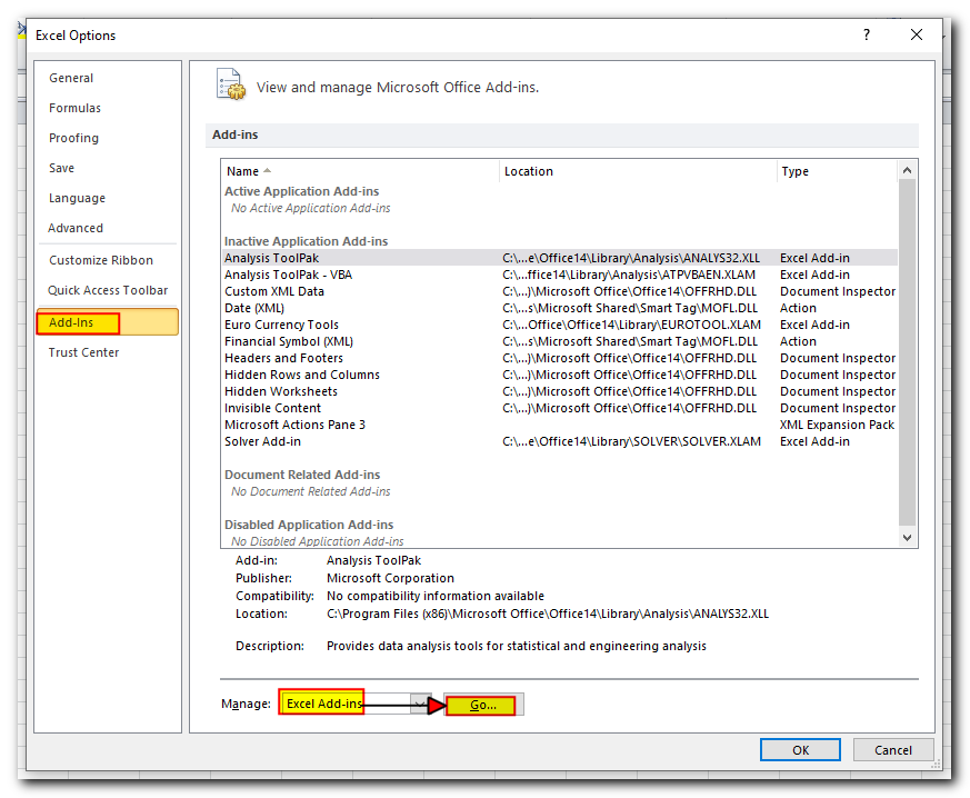
- In the Excel Options window, click Add-Ins on the left side. Make sure Excel Add-ins is selected in the “Manage” box at the bottom, and then click Go
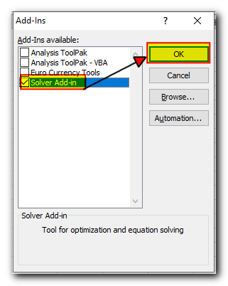
- In the Add-Ins dialog box, check the Solver Add-in box, and click OK:
To get Solver on Excel 2003, go to the Tools menu, and click Add-Ins. In the Add-Ins available list, check the Solver Add-in box, and click OK.
Where is Solver in Excel?
In the modern versions of Excel, the Solver button appears on the Data tab, in the Analysis group:

How to use Solver in Excel
Before using the Excel Solver add-in, you need to set up the problem you want to solve in a worksheet. Here’s an example of how to solve a simple optimization problem.
Problem: Imagine you own a beauty salon, and you’re planning to offer a new service. You need to buy new equipment that costs $40,000, and you’ll be paying for it in monthly installments over 12 months.
Goal: Find the lowest price you can charge for the service that will allow you to pay for the new equipment within the 12-month period.
For this, I’ve created the following model:
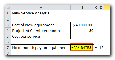
And now, let’s see how Excel Solver can find a solution for this problem.
1. Run Excel Solver
On the Data tab, in the Analysis group, click the Solver button.
2. Define the problem
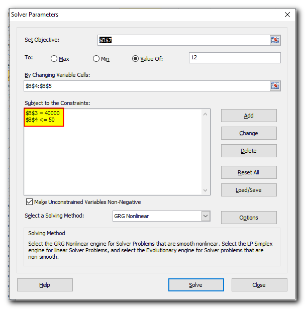
The Solver Parameters window will open, where you’ll need to set up three main parts:
- Objective cell
- Variable cells
- Constraints
What does Excel Solver do with these? It finds the best solution (whether it’s a maximum, minimum, or a specific value) for the formula in the Objective cell by adjusting the values in the Variable cells. It does this while following the rules or limits you set in the Constraints cells.
Objective
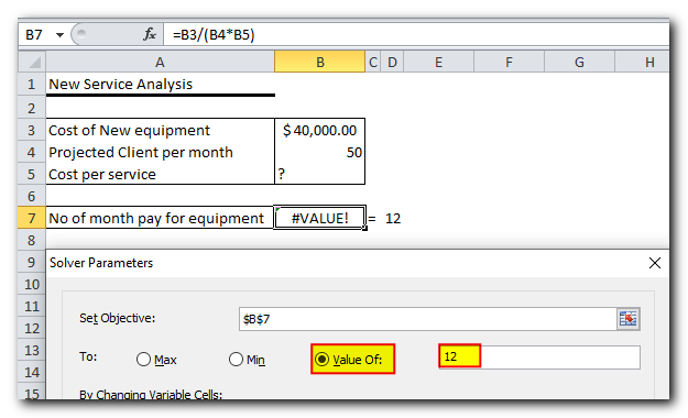
The Objective cell (called Target cell in older versions of Excel) is the cell with the formula that represents the goal of your problem. Your goal could be to maximize, minimize, or reach a specific value.
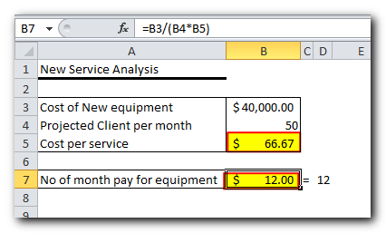
In this example, the Objective cell is B7, which calculates the payment term using the formula =B3/(B4*B5). The result of this formula should equal 12
Variable cells
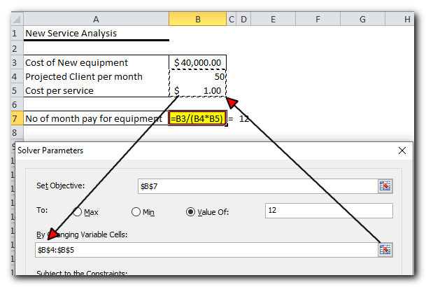
Variable cells (called Changing cells or Adjustable cells in older versions) are the cells with data that can be changed to reach your goal. Excel Solver lets you choose up to 200 variable cells.
In this example, we have two variable cells:
- Projected clients per month (B4), which should be 50 or less.
- Cost per service (B5), which we want Excel Solver to figure out.
Constraints
Excel Solver Constraints are the limits or rules for the possible solutions to your problem. In other words, they are the conditions that must be followed.
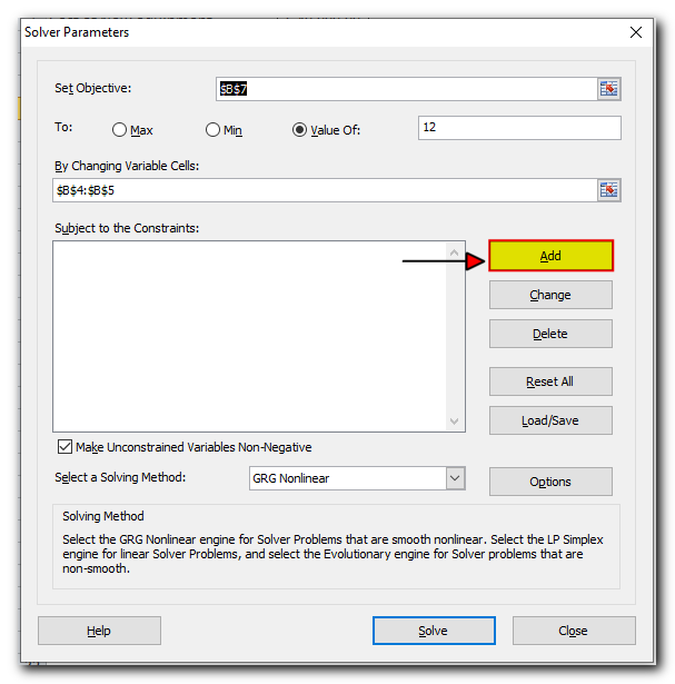
To add a constraint, follow these steps:
- Click the Add button next to the “Subject to the Constraints” box.
- In the Constraint window, enter a constraint.
- Click the Add button to add the constraint to the list.
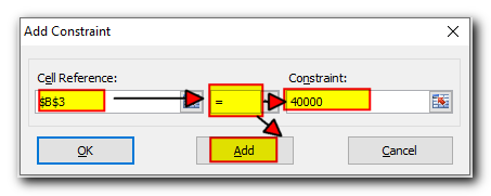
Keep adding any other constraints as needed. Once you’ve entered the last constraint, click OK to go back to the main Solver Parameters window.
Excel Solver allows you to set the following relationships between a cell and its constraint:
- Less than or equal to, equal to, or greater than or equal to: In the Cell Reference box, select a cell, choose one of these signs: <=, =, or >=, and enter a number, cell reference, or formula in the Constraint
- Integer: If the cell must be a whole number, choose int, and “integer” will show up in the Constraint box.
- Different values: If each cell in a range must have a unique value, select dif, and “AllDifferent” will appear.
- Binary: To limit a cell to either 0 or 1, choose bin, and “binary” will appear in the Constraint box
Note: The int, bin, and dif relationships can only be applied to Variable cells.
To edit or delete a constraint, follow these steps:
- In the Solver Parameters window, click on the constraint you want to change.
- To edit it, click Change and make your changes.
- To delete it, click the Delete button.
In this example, the constraints are:
- B3 = 40000 – the cost of the new equipment is $40,000.
- B4 <= 50 – the number of projected clients per month is less than or equal to 50.
3. Solve the problem
After setting up all the parameters, click the Solve button at the bottom of the Solver Parameters window (as shown in the screenshot). This will let Excel Solver work on finding the best solution for your problem.
The time Solver takes to find the solution depends on how complex your model is, as well as your computer’s memory and processor speed. It might take a few seconds, minutes, or even hours.
When Solver finishes, it will show the Solver Results dialog box. Choose Keep the Solver Solution and then click OK
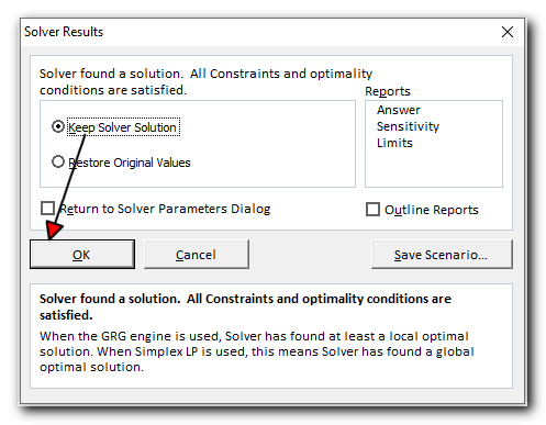
The Solver Result window will close and the solution will appear on the worksheet right away.
In this example, $66.67 appears in cell B5, which is the minimal cost per service that will let you pay for the new equipment in 12 months, provided there are at least 50 clients per month:
Excel Solver examples
Below you will find two more examples of using the Excel Solver addin. First, we will find a solution for a well-known puzzle, and then solve a real-life linear programming problem.
Excel Solver example 1 (magic square)
Most people are familiar with “magic square” puzzles, where you place numbers in a square so that all the rows, columns, and diagonals add up to the same number.
For example, do you know how to solve a 3×3 magic square using the numbers 1 to 9, where each row, column, and diagonal adds up to 15?
You could solve this puzzle by trial and error, but the Solver tool will likely find the solution much faster. Our task is to set up the problem correctly.
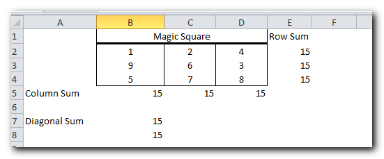
First, enter the numbers 1 to 9 in a 3×3 table. Excel Solver doesn’t actually need these numbers to work, but they’ll help us see the problem. What Solver really needs are SUM formulas that add up each row, column, and the two diagonals

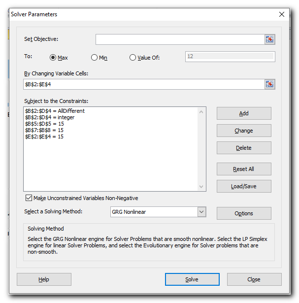
With all the formulas in place, run Solver and set up the following parameters:
- SetObjective. In this example, we don’t need to set any objective, so leave this box empty.
- Variable Cells. We want to populate numbers in cells B2 to D4, so select the range B2:D4.
- Constraints. The following conditions should be met:
- $B$2:$D$4 = AllDifferent – all of the Variable cells should contain different values.
- $B$2:$D$4 = integer – all of the Variable cells should be integers.
- $B$5:$D$5 = 15 – the sum of values in each column should equal 15.
- $E$2:$E$4 = 15 – the sum of values in each row should equal 15.
$B$7:$B$8 = 15 – the sum of both diagonals should equal 15.
Finally, click the Solve button, and the solution is there!
How to save and load Excel Solver scenarios
When solving a problem, you might want to save your Variable cell values as a scenario that you can look at or use later.
For example, when calculating the lowest service cost in the first example of this tutorial, you might want to test different numbers of projected clients per month and see how it changes the service cost. You may also want to save the most likely scenario you’ve already worked out, so you can bring it back anytime.
Saving an Excel Solver scenario is as simple as choosing a range of cells to store the data. Loading a Solver model is just about telling Excel which range of cells holds your saved model. The detailed steps are below
Saving the model
To save the Excel Solver scenario, perform the following steps:
- Open the worksheet with the calculated model and run the Excel Solver.
- In the Solver Parameters window, click the Load/Save
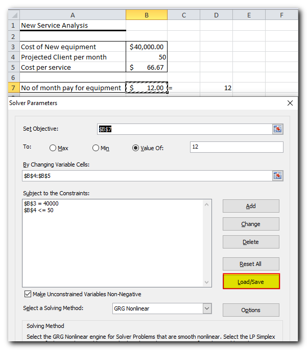
3.Excel Solver will tell you how many cells are needed to save your scenario. Select that many empty cells and click Save:
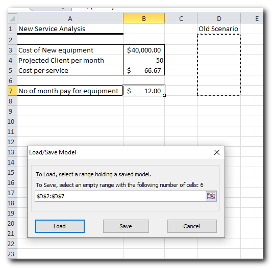
4.Excel will save your current model, which may look something similar to this:
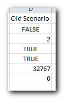
At the same time, the Solver Parameters window will show up where you can change your constraints and try different “what if” options.
Loading the saved model
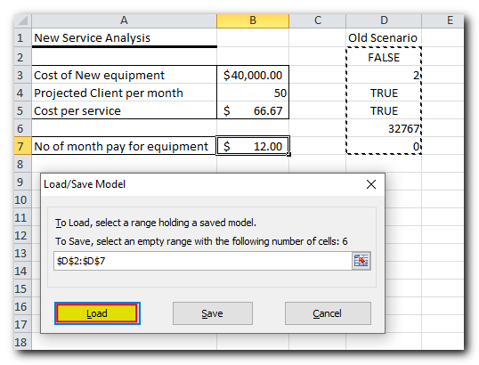
When you decide to restore the saved scenario, do the following:
- In the Solver Parameterswindow, click the Load/Save
- On the worksheet, select the range of cells holding the saved model and click Load:
In the Load Model dialog, click the Replace button:
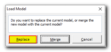
This will open the main Excel Solver window with the parameters of the previously saved model. All you need to do is to click the Solve button to re-calculate it.
Excel Solver algorithms
When setting up a problem in Excel Solver, you can choose from the following methods in the Select a Solving Method dropdown:
- GRG Nonlinear: This method uses the Generalized Reduced Gradient Nonlinear algorithm for problems with smooth nonlinear constraints. This means that at least one of the conditions depends on a smooth nonlinear formula. More details are available here.
- LP Simplex: This method is based on the Simplex algorithm developed by George Danzig. It is used for solving Linear Programming problems, where the goal is to maximize or minimize a single objective represented by a linear equation. More information can be found here.
- Evolutionary: This method is for non-smooth problems, which are harder to solve because some functions are irregular or even have breaks, making it difficult to find out if a function is increasing or decreasing. For more details, check this page.
To adjust how Solver finds the solution, click the Options button in the Solver Parameters window and set your preferences on the GRG Nonlinear, All Methods, or Evolutionary tabs.
This is how you can use Solver in Excel to find the best solutions for your decision problems. At the end of this tutorial, you can download a sample workbook with all the examples to help you understand better. Thanks for reading, and I hope to see you on our blog next week!
 New Excel VBA Course Live Now! $49 for first 100 Students Only


