ROMAN Function In Excel
The ROMAN function in Excel converts numbers into Roman numerals. It’s useful when you need to display numbers in the Roman numeral format, such as for dates, titles, or other specific purposes. The function allows you to choose how “traditional” or simplified the Roman numeral should be. To use the ROMAN function, you just need to enter the number you want to convert, and Excel will do the rest
Table of Contents
When to Use ROMAN Function in Excel
The ROMAN Function changes regular numbers (Arabic Numbers) into Roman Numerals. In the Roman Numeral system, specific symbols are used to represent numbers.
Roman Numeral | Number |
I | 1 |
V | 5 |
X | 10 |
L | 50 |
C | 100 |
D | 500 |
M | 1000 |
Using these 7 Roman Numerals, we can convert any Arabic number into a value of the ancient Roman Number System and vice versa.
Syntax and Arguments
=ROMAN(number,[form])
The following points contain important information regarding the inputs required by ROMAN Function in Excel.
- number – This is the Arabic numerical value that we want to convert to the Roman number system.
- [form] – This is an optional argument. Its value ranges from 0 to 4. It specifies the Roman Numeral abbreviation and how concise would be the result
Important Points about ROMAN Function
There are some important notes about the ROMAN Function that you must remember.
Range: It can only convert numbers from 0 to 4000. If you enter a number outside this range, like more than 3999 or less than 0, you’ll get a #VALUE! error.
Whole Numbers Only: You need to use whole numbers (no decimals). Any decimal part will be ignored.
Reversing the Conversion: To change Roman numerals back to Arabic numbers, use the ARABIC Function.
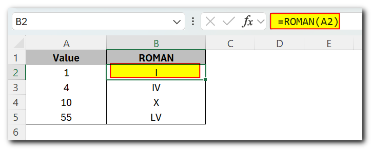
Let us suppose we have some numerical value in range A2:A5
Use the following ROMAN function formula in Cell B2 and copy it down.
=ROMAN(A2)
Examples for ROMAN Function in Excel
In this part of the blog, we are going to implement the ROMAN Function in practice.
Example 1 – Basic Example for ROMAN Formula
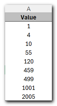
Let us suppose we have got the following values in the range A2:A10
Use the following ROMAN Formula to get the ROMAN Numerals for the Data.
=ROMAN(A2)
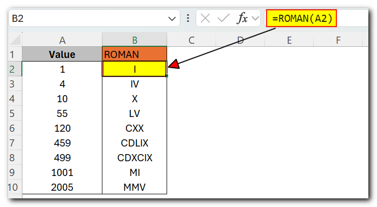
We have entered the formula in cell B2. Select the range B2:B10 and press the ctrl d key to copy the formula for all of the numerical values. As a result, we got the data converted into Roman numerals.
Example 2 – Using Different Forms in ROMAN function
By using the “form” argument, we can choose different styles for the ROMAN Function. The “form” argument can be set to 0, 1, 2, 3, or 4, depending on how simple or detailed we want the Roman numeral to be. For example, if we want to convert the number 499 into different Roman numeral styles, we can adjust the “form” argument accordingly
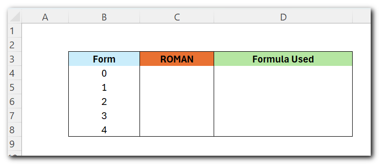
We have entered different forms in column B. Enter the following formula in cell C3 and copy it down the range C3:C7.
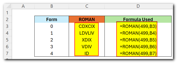
As a result, we got 499 converted into different ROMAN Numeral forms.
Explanation: We used the number 499 directly in the formula, so it stays the same when you copy the formula down. The “form” input is a reference to cell B3, which contains the value 0. This means that the number 499 is converted to the default Roman numeral style.
When we copy down the formula, the form corresponding to each cell would be considered and we will get a more concise conversion.
This brings us to the end of the ROMAN Function blog.
Feel free to contact us in case of any concern


