Offset Function in Excel
In this tutorial, we’re going to explore one of the most intriguing features in Excel: the OFFSET function.
So, what is the OFFSET function in Excel? Simply put, OFFSET gives you a reference to a range of cells that’s moved from a starting point by a certain number of rows and columns.
The OFFSET function might seem a bit complicated at first, so let’s start with a simple explanation of how it works. After that, we’ll look at some of the best ways to use OFFSET in Excel.
Table of Contents
Excel OFFSET function - syntax and basic uses
The OFFSET function in Excel returns a cell or range of cells that is a given number of rows and columns from a given cell or range.
The syntax of the OFFSET function is as follows:
OFFSET(reference, rows, cols, [height], [width])
The first 3 arguments are required and the last 2 are optional. All of the arguments can be references to other cells or results returned by other formulas.
It looks like Microsoft made a good effort to put some meaning into the parameters’ names, and they do give a hint at what you are supposed to specify in each.
Required arguments:
**Reference:** This is the cell or group of cells where you start. Think of it as your starting point.
**Rows:** This tells you how many rows to move up or down from your starting point. If the number is positive, you move down. If it’s negative, you move up.
**Cols:** This tells you how many columns to move left or right from your starting point. Positive numbers move to the right, while negative numbers move to the left.
Optional arguments:
- Height– the number of rows to return.
- Width– the number of columns to return.
Both the height and width arguments must always be positive numbers. If either is omitted, it defaults to the height or width of reference.
Note. OFFSET is a volatile function and may slow down your worksheet. The slowness is directly proportional to the number of cells recalculated.
And now, let’s illustrate the theory with an example of the simplest OFFSET formula.
Excel OFFSET formula example
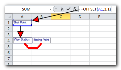
=OFFSET(A1,3,1)
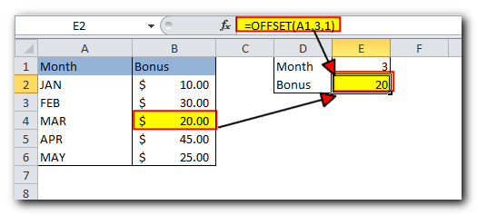
This formula tells Excel to start at cell A1 (our reference point), then move 3 rows down and 1 column to the right. So, it points to cell B4.
In the image on the left, you can see how the formula works. On the right, there’s another OFFSET formula that’s almost the same, but it uses a cell reference (E1) for the rows argument. Since E1 has the number 3, just like the first formula, both formulas end up pointing to the same cell: B4.
Excel OFFSET formulas - things to remember
The OFFSET function in Excel doesn’t actually move cells or ranges; it just creates a reference to a different cell or range.
- When OFFSET returns a range of cells, the row and column numbers you specify always start from the top-left cell of that range.
- The reference you use with OFFSET must include at least one cell or a group of adjacent cells. If it doesn’t, the formula will show a #VALUE! error.
- If the rows or columns you specify move the reference outside the limits of the spreadsheet, OFFSET will return a #REF! error.
- You can use OFFSET within other Excel functions that require a cell or range reference.
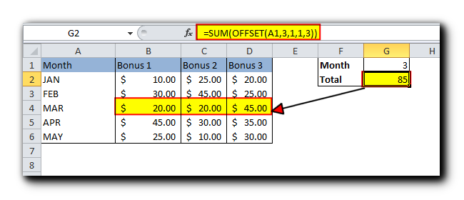
For example, in older versions of Excel (2019 and earlier), the formula OFFSET(A1,3,1,1,3) would result in a #VALUE! error because it tries to return a range (1 row and 3 columns) that doesn’t fit into a single cell. However, if you use OFFSET within the SUM function like this:
=SUM(OFFSET(A1,3,1,1,3))
It will correctly calculate the sum of the values in a range of 1 row by 3 columns, which is located 3 rows below and 1 column to the right of cell A1 (i.e., the total of values in cells B4).
In situation when you wish to base the offset from the current cell, you can use the INDIRECT and ADDRESS functions in combination with ROW() and COLUMN() to get the starting reference. For example:
=SUM(OFFSET(INDIRECT(ADDRESS(ROW(), COLUMN())), 3, 1, 1, 3))
Why do I use OFFSET in Excel?
You might wonder why you should use the OFFSET function instead of just writing a direct reference like B4
. Here’s why OFFSET can be useful:
- Creating Dynamic Ranges: Fixed references like B1
always point to the same cells. OFFSET lets you create dynamic ranges that adjust automatically as your data changes. This is especially helpful if your data grows or changes, like when new rows or columns are added regularly.
2. Flexible Range Sizing: If you don’t know the exact address of the range but know where it starts, OFFSET helps by allowing you to define the range based on a starting cell. This flexibility makes it easier to work with data that changes or shifts
How to use OFFSET function in Excel - formula examples
I hope you haven’t get bored with that much of theory. Anyway, now we are getting to the most exciting part – practical uses of the OFFSET function.
Excel OFFSET and SUM functions
The example we discussed a moment ago demonstrates the simplest usage of OFFSET & SUM. Now, let’s look at these functions at another angle and see what else they can do.
Example 1. A dynamic SUM / OFFSET formula
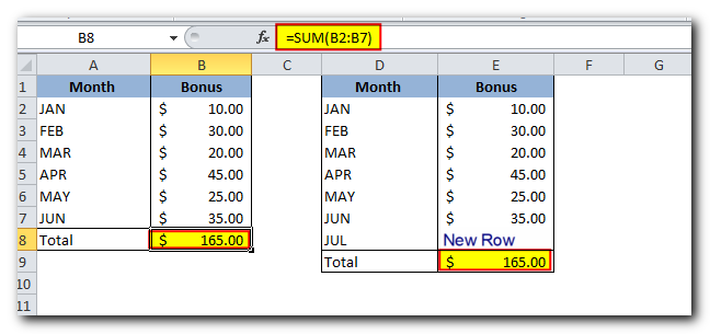
When you work with a worksheet that gets updated regularly, you might want a SUM formula that automatically includes any new rows you add.
For example, imagine you have a table of data like in the screenshot below. Each month, you add a new row just above the SUM formula, and you want that new row to be included in the total. You have two options: either manually update the range in the SUM formula every time you add a new row, or use the OFFSET formula to do it automatically
In the SUM formula, you’ll directly specify the first cell of the range you want to sum. The next step is to figure out the parameters for the Excel OFFSET function, which will find the last cell in that range:
- Reference: This is the cell that holds the total, which is B9 in our example.
- Rows: This is the cell right above the total, so you’ll use -1 because it’s one row up.
- Cols: This is 0 because you don’t want to move to a different column.
Now, here’s how the SUM/OFFSET formula looks
=SUM(first cell:(OFFSET(cell with total, -1,0)
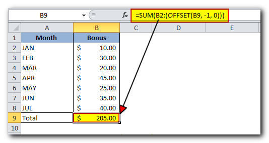
Tweaked for the above example, the formula looks as follows:
=SUM(B2:(OFFSET(B9, -1, 0)))
And as demonstrated in the below screenshot, it works flawlessly
Example 2. Excel OFFSET formula to sum the last N rows
In the example above, let’s say you want to find out the total bonuses for the last N months, instead of calculating the grand total for all months. You also want the formula to automatically update if you add new rows to your sheet.
To achieve this, we’ll use Excel’s OFFSET function together with the SUM and COUNT (or COUNTA) functions.
Here are two formula options:
=SUM(OFFSET(B1,COUNT(B:B)-E1+1,0,E1,1)) =SUM(OFFSET(B1,COUNTA(B:B)-E1,0,E1,1))
In simpler words, these formulas will calculate the sum of the bonuses for the last N months, and if you add new data, the formula will include that automatically.
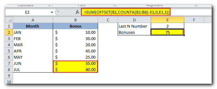
Here’s a breakdown of the formulas in simple terms:
- Reference: This is the starting point, which is the header of the column you want to sum. In this example, it’s cell B1.
- Rows: To figure out how many rows to skip (or “offset”), you use either the COUNT or COUNTA function.
- COUNT: This function counts the number of cells in column B that contain numbers. You subtract the number in E1 (representing the last N months) and add 1 to include the most recent month.
- COUNTA: If you use COUNTA (which counts all non-empty cells, including text), you don’t need to add 1. This is because it already includes the header row, which has text. This formula works best with tables that have one header row followed by rows with numbers. For other table layouts, you might need to adjust the formula.
- Cols: This represents how many columns to skip. Here, it’s 0, meaning no column offset is needed.
- Height: This is the number of rows you want to sum, which is given by the value in E1.
- Width: This is set to 1 column because you’re summing values from one column.
In summary, these details explain how each part of the formula works to sum the last N months and adjust when new rows are added.
Using OFFSET function with AVERAGE, MAX, MIN
Just like we calculated the bonuses for the last N months, you can also find the average, maximum, or minimum for the last N days, weeks, or years. The only thing that changes in the formulas is the name of the first function:
average, use: =AVERAGE(OFFSET(B1,COUNT(B:B)-E1+1,0,E1,1)) maximum,use:=MAX(OFFSET(B1,COUNT(B:B)-E1+1,0,E1,1)) minimum,use:=MIN(OFFSET(B1,COUNT(B:B)-E1+1,0,E1,1))
In simple terms, these formulas work the same way, but instead of summing, they calculate the average, highest, or lowest value for the last N entries
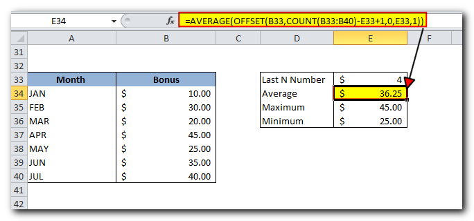
The main advantage of using these formulas instead of regular ones like AVERAGE(B5) or MAX(B5) is that you don’t need to update the formula every time you change your table. Whether you add or delete rows, the OFFSET formulas will always look at the last few cells in the column based on the number you specify. This means the formulas automatically adjust to include the most recent data without any extra work from you.
Excel OFFSET formula to create a dynamic range
Used in conjunction with COUNTA, the OFFSET function can help you make a Dynamic Range that may prove useful in many scenarios, for example to create automatically updatable drop-down lists.
The OFFSET formula for a dynamic range is as follows:
=OFFSET(Sheet_Name!$A$1, 0, 0, COUNTA(Sheet_Name!$A:$A), 1)
At the heart of this formula, you use the Counta Function to get the number of non-blank cells in the target column. That number goes to the height argument of OFFSET instructing it how many rows to return.
Apart from that, it’s a regular Offset formula, where:
Reference is the starting point from which you base the offset, for example Sheet1!$A$1.
Rows and Cols are both 0 because there are no columns or rows to offset.
Width is 1 column.
Note. If you are making a dynamic range in the current sheet, there is no need to include the sheet name in the references, Excel will do it for you automatically when creating the named range. Otherwise, be sure to include the sheet’s name followed by the exclamation point like in this formula example.
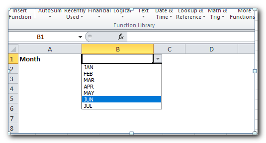
Once you’ve created a dynamic named range with the above OFFSET formula, you can use Data Validation to make a dynamic dropdown menu that will update automatically as soon as you add or remove items from the source list.
Excel OFFSET & VLOOKUP
As many people know, VLOOKUP is used for looking up data vertically, and HLOOKUP is used for looking up data horizontally in Excel. However, these functions have some limitations and may not work well for more complex tasks. To do more advanced searches in your Excel tables, it’s better to use functions like INDEX, MATCH, or OFFSET
Example 1. OFFSET formula for a left Vlookup in Excel
One of the biggest limitations of the VLOOKUP function is that it can’t look to the left. VLOOKUP can only find values to the right of the column you’re searching in.
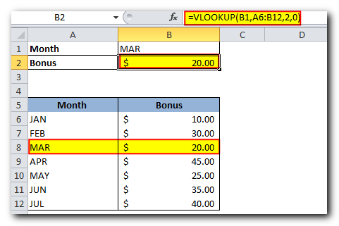
For example, in our lookup table with two columns – month names (column A) and bonuses (column B) – you can easily find the bonus for a specific month using this formula:
=VLOOKUP(B1, A5, 2, FALSE)
But if you switch the columns around, the formula will give you an #N/A error.
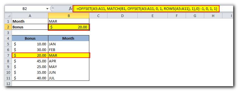
To perform a left-side lookup, you need a more flexible function that can work no matter where the return column is. One solution is to use the INDEX and MATCH functions together. Another option is to use OFFSET, MATCH, and ROWS
OFFSET(lookup_table, MATCH(lookup_value, OFFSET(lookup_table, 0, lookup_col_offset, ROWS(lookup_table), 1) ,0) -1, return_col_offset, 1, 1)
Where:
- Lookup_col_offset is the number of columns to move from the starting point to the column you’re searching in.
- Return_col_offset is the number of columns to move from the starting point to the column you’re returning a value from.
In our example, the lookup table is A5
, and the value we are searching for is in cell B1. The lookup column offset is 1 (because we’re searching in the second column, B, so we move 1 column to the right). The return column offset is 0 because we’re returning values from the first column, A.
Here’s the formula:
=OFFSET(A5, MATCH(B1, OFFSET(A5, 0, 1, ROWS(A5), 1), 0) – 1, 0, 1, 1)
It might look a bit tricky, but it works
Example 2. Two-way lookup (by column and row values)
A two-way lookup finds a value by matching both rows and columns. You can use the following array formula to find the value where a specific row and column meet.
=OFFSET(lookup table, MATCH(row lookup value, OFFSET(lookup table, 0, 0, ROWS(lookup table), 1), 0) -1, MATCH(column lookup value, OFFSET(lookup table, 0, 0, 1, COLUMNS(lookup table)), 0) -1)
Given that:
- The lookup table is A5
- The value to match in the rows is in B2
- The value to match in the columns is in B1
The two-dimensional lookup formula would be:
=OFFSET(A5, MATCH(B2, OFFSET(A5, 0, 0, ROWS(A5), 1), 0) – 1, MATCH(B1, OFFSET(A5, 0, 0, 1, COLUMNS(A5)), 0) – 1)
It’s not the easiest formula to remember, right? Also, since this is an array formula, make sure to press Ctrl + Shift + Enter to use it correctly

Of course, this long OFFSET formula isn’t the only way to do a two-way lookup in Excel. You can get the same result using other methods like VLOOKUP with MATCH, SUMPRODUCT, or INDEX with MATCH. There’s even a way to do it without formulas by using named ranges and the intersection operator (a space). The following tutorial explains all these alternative solutions in detail: How to do a two-way lookup in Excel.
Do you remember the question asked at the beginning of this tutorial – What is OFFSET in Excel? I hope now you know the answer : ) If you want some more hands-on experience, feel free to download our practice workbook (please see below) containing all the formulas discussed on this page and reverse engineer them for deeper understanding. Thank you for reading!


