How to calculate NPV in Excel
In this guide, you will learn how to Calculate the NPV in Excel the net present value of an investment and how to avoid common mistakes when using NPV in Excel.
Net present value (NPV) is an important part of financial analysis. It helps you figure out if a project will make a profit or not. Why is NPV so important? The main idea is that money you might get in the future is worth less than the same amount of money you have today. NPV adjusts future cash flows to show what they’re worth today.
Excel has a built-in NPV function to help with this, but it can be tricky, especially for beginners in financial modeling. This article will explain how to use the Excel NPV function and highlight common errors you should avoid when calculating NPV for a series of cash flows
Table of Contents
What is net present value (NPV)?
Net present value (NPV) is the total value of a series of cash flows from a project, but adjusted to what they are worth today.
In simple terms, NPV is the value of future cash flows minus the cost of the initial investment:
NPV = Present value of future cash flows – Initial Investment
To understand this better, let’s take a closer look at the math behind it.
For a single cash flow, the present value (PV) is calculated using this formula:
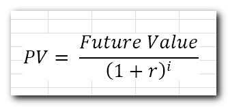
Where:
- r – discount or interest rate
- i – the cash flow period
For example, to get $110 (future value) after 1 year (i), how much should you invest today in your bank account which is offering 10% annual interest rate (r)? The above formula gives this answer:
$110/(1+10%)^1 = $100
In other words, $100 is the present value of $110 that are expected to be received in the future.
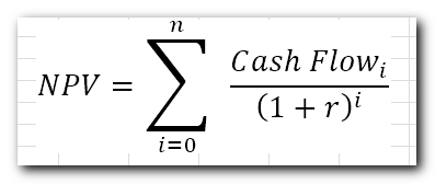
Net present value (NPV) adds up the present values of all future cashflows to bring them to a single point in present. And because the idea of “net” is to show how profitable the project is going to be after accounting for the initial capital investment required to fund it, the amount of initial investment is subtracted from the sum of all present values:

Where:
- r – discount or interest rate
- n – the number of time periods
- i – the cash flow period
Because any non-zero number raised to the zero power equals 1, we can include the initial investment in the sum. Please notice, that in this compact version of the NPV formula, i=0, i.e. the initial investment is made in period 0.
For example, to find NPV for a series of cash flows (50, 60, 70) discounted at 10% and the initial cost of $100, you can use this formula:

Or

How does net present value (NPV) help in deciding if an investment is a good idea? The basic idea is that if the NPV is positive, the investment is expected to make a profit. If the NPV is negative, the investment will likely lose money. This is known as the Net Present Value Rule, which says you should only take on projects with a positive NPV, as they are more likely to be profitable.
Excel NPV function
The NPV function in Excel returns the net present value of an investment based on a discount or interest rate and a series of future cash flows.
The syntax of the Excel NPV function is as follows:
NPV(rate, value1, [value2], …)
Where:
- Rate (required) – the discount or interest rate over one period. It must be supplied as percentage or a corresponding decimal number.
- Value1, [value2], …– numeric values representing a series of regular cash flows. Value1is required, subsequent values are optional. In the modern versions of Excel 2007 to 2019, up to 254 value arguments can be supplied; in Excel 2003 and older – up to 30 arguments.
The NPV function is available in Excel 365 – 2000.
4 things you should know about NPV function
To make sure your NPV formula in Excel works properly, keep these things in mind:
- Cash flows should happen at the end of each period. If the first cash flow (like the initial investment) happens at the start of the first period, use a special NPV formula.
- Enter the cash flow values in order, from first to last, and make sure they are spaced evenly over time.
- Use negative numbers for money going out (expenses) and positive numbers for money coming in (income).
- Only numbers are used in the calculation. Empty cells, text, logical values (like TRUE/FALSE), or error messages are ignored.
How Excel NPV function works
Using the NPV function in Excel can be a bit tricky because of how the function is set up. By default, Excel assumes that the investment is made one period before the first cash flow date. This means that the NPV formula works correctly only if you enter the initial investment cost as happening one period in the future, not today!
To illustrate this, let’s calculate net present value manually and with an Excel NPV formula, and compare the results.
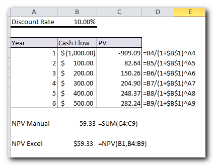
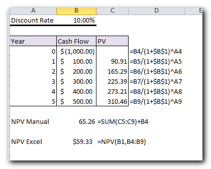
Let’s say, you have a discount rate in B1, a series of cash flows in B4:B9 and period numbers in A4:A9.
Supply the above references in this generic PV formula:
PV = future value/(1+rate)^period
And you will get the following equation:
=B4/(1+$B$1)^A4
This formula is entered in cell C4 and then copied to the cells below. Thanks to the smart use of absolute and relative cell references, the formula automatically adjusts for each row, as shown in the screenshot below.
Also, notice that we calculate the present value of the initial investment since it happens after 1 year. Because of this, it is discounted as well.
After that, we add up all the present values to get the total.
=SUM(C4:C9)
And now, let’s do NPV with the Excel function:
=NPV(B1, B4:B9)
As you can see, the results of both calculations match exactly:
But what if the initial investment happens at the start of the first period, like it usually does?
Since the investment is made today, it doesn’t need to be discounted. So, you just add this amount to the total of the present values of future cash flows. Since the initial investment is a negative number (money going out), it’s actually subtracted from the sum:
=SUM(C4)+B4
In this case, the result from this manual calculation will be different from the result given by Excel’s NPV function.
Does this mean we cannot rely on the NPV formula in Excel and have to calculate net present value manually in this situation? Of course, not! You will just need to tweak the NPV function a little as explained in the next section.
How to calculate NPV in Excel
When the initial investment is made at the start of the first period, we can treat it as a cash flow at the end of the previous period (i.e. period 0). With that in mind, there are two simple ways to find NPV in Excel.
Excel NPV formula 1
Leave the initial cost out of the range of values and subtract it from the NPV function’s result. Since the initial outlay is typically entered as a negative number, you actually perform the addition operation:
NPV(rate, values) + initial cost
In this case, the Excel NPV function just returns the present value of uneven cash flows. Because we want “net” (i.e. present value of future cash flows less initial investment), we subtract the initial cost outside of the NPV function.
Excel NPV formula 2
Include the initial cost in the range of values and multiply the result by (1 + rate).
When using the NPV function in Excel, it assumes the initial investment was made one period before the first cash flow (period -1). To correct this and bring the NPV forward to the current period (i.e., from period -1 to period 0), you need to multiply the result by (1 + r), where “r” is the discount rate. This adjusts the NPV to reflect the present time.
Here’s the more compact form of the NPV formula.
NPV(rate, values) * (1+rate)
Which formula to use is a matter of your personal preference. I personally believe the first one is simpler and easier to understand
NPV calculator in Excel
Now let’s see how you can use the formulas mentioned above with real data to create your own NPV calculator in Excel.
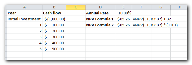
Suppose you have: The initial investment in B2,A series of future cash flows in B3,And the required return rate in F1.
To calculate the NPV, you can use one of these formulas:
NPV Formula 1:
=NPV(F1, B3:B7) + B2
Here, the first cash flow (in B3) starts at period 1, and the initial investment (B2) is added separately, not included in the range.
NPV Formula 2:
=NPV(F1, B2:B7) * (1+F1)
This formula includes the initial investment (B2) in the range, and we multiply the result by (1 + F1) to adjust for the correct time period.
The screenshot below shows how this NPV calculator works in Excel.
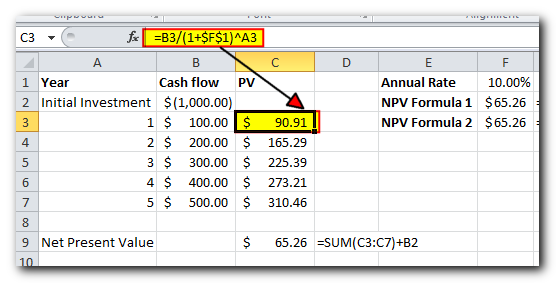
To make sure our Excel NPV formulas are correct, let us check the result with manual calculations.
First, we find the present value of each cash flow by using the PV formula discussed above:
=B3/(1+$F$1)^A3
Next, add up all the present values and subtract the initial cost of investment:
=SUM(C3:C7)+B2
… and see that the results of all three formulas are absolutely the same.
Difference between PV and NPV in Excel
In finance, both PV (Present Value) and NPV (Net Present Value) are used to measure the current value of future cash flows by bringing future amounts back to the present. However, there’s one key difference:
- Present Value (PV): This refers to the value of all future cash inflows for a specific period.
- Net Present Value (NPV): This is the difference between the present value of cash inflows and cash outflows (like the initial investment).
In simple terms, PV only looks at the money coming in, while NPV also subtracts the initial investment, giving a more complete “net” value.
In Microsoft Excel, there are two important differences between the NPV and PV functions:
- The NPV function can handle uneven (changing) cash flows. The PV function needs the cash flows to be the same throughout the investment period.
- For NPV, cash flows must occur at the end of each period. With PV, cash flows can happen either at the end or the beginning of a period.
That’s how to use NPV in Excel to find the net present value of an investment. To have a closer look at the formulas discussed in this tutorial, please feel free to download our sample
Thank you for reading and hope to see you on our blog next week!


