Lock a Column in Excel – 3 Easy and Simple Methods
Microsoft Excel lets you share your spreadsheets with others, but sometimes your co-workers might edit the wrong column by mistake. To avoid this, you can lock specific columns.
In this guide, we’ll show you how to lock a column in Excel so you don’t have to worry about mistakes.
Method 1:- Lock a column in Excel Using Context Menu
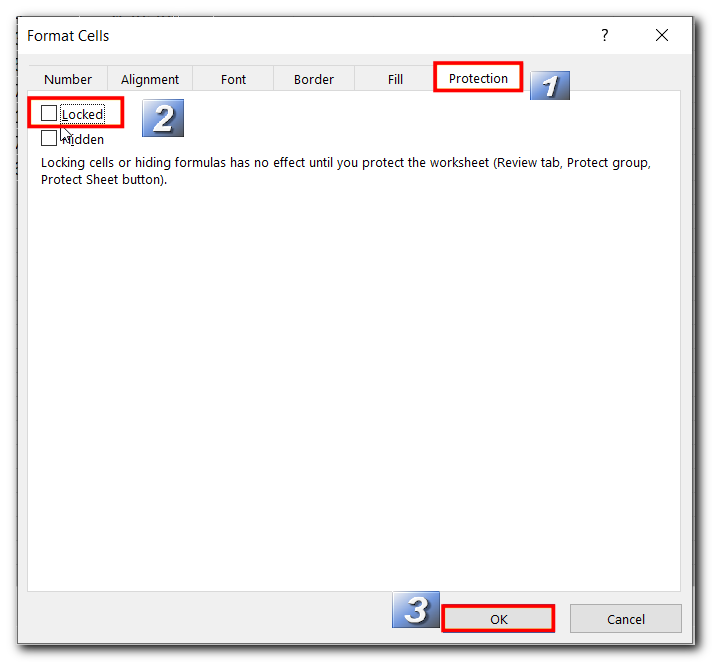
- Go to the Protection tab and uncheck the “Locked” option. Then, click OK. This will unlock all the cells in the spreadsheet.
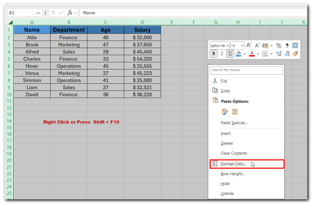
- Go back to your spreadsheet and select the columns you want to lock.
- Open the context menu. Select the Format Cells option.
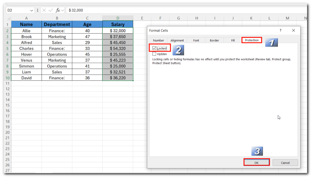
- Check the Locked option in the Protection tab from the Format Cells box.
- Click on OK.
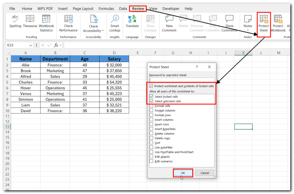
- Select the Review tab from your ribbon.
- Select Protect Sheet from the Protect group.
- A “Protect Sheet” box will appear. Ensure the “Protect worksheet and contents of locked cells” option is checked. Enter a password (if you want) in the password field and click OK.
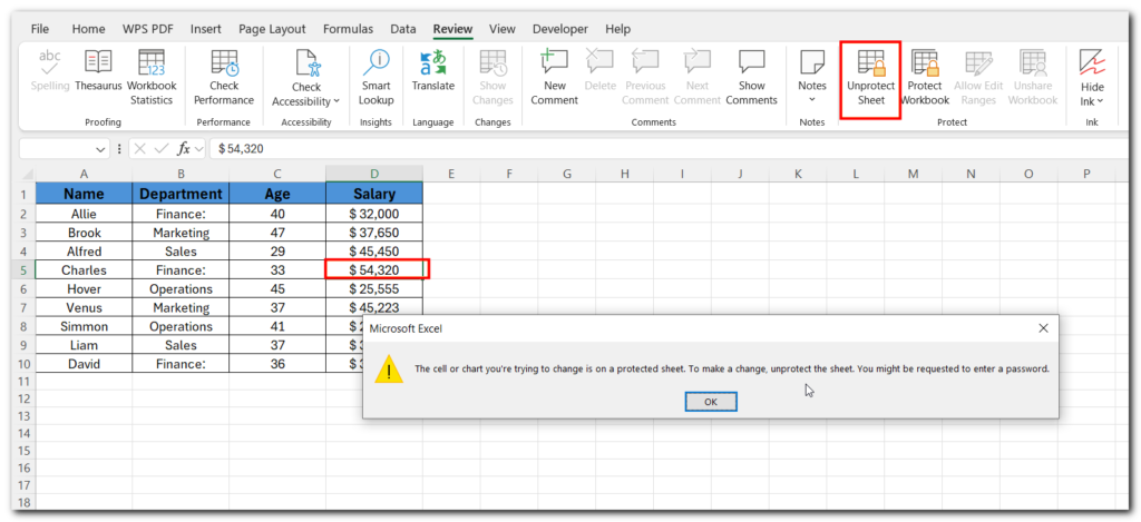
From now on, a warning box will pop up, stopping anyone from editing the selected columns. To make changes, you’ll need to unprotect the sheet first.
Method 2 :– Lock a Column in Excel Using the Dialog Box Launcher
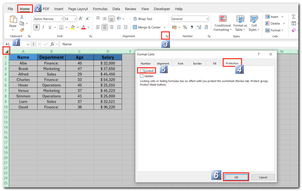
- Click the small triangle where the row headers and column headers meet to select all the cells in the spreadsheet.
- Open the dialog box launcher by clicking the small downward-right arrow next to the group names in the Home tab.
- The Format Cells box will open. Go to the Protection tab and uncheck the Locked box.
- Click on OK.
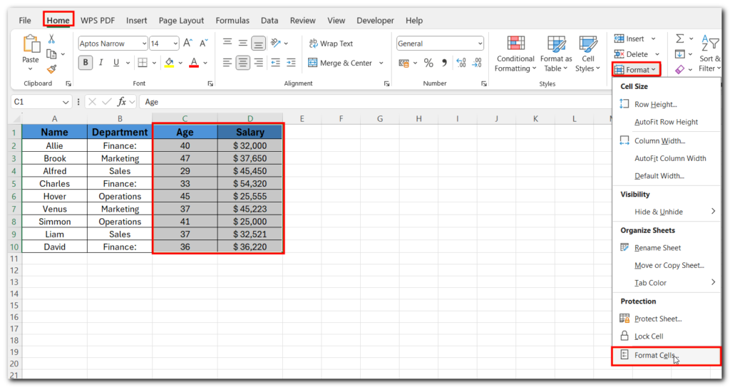
- Select the columns you want to protect by clicking the column letters
- Open Format Cells.
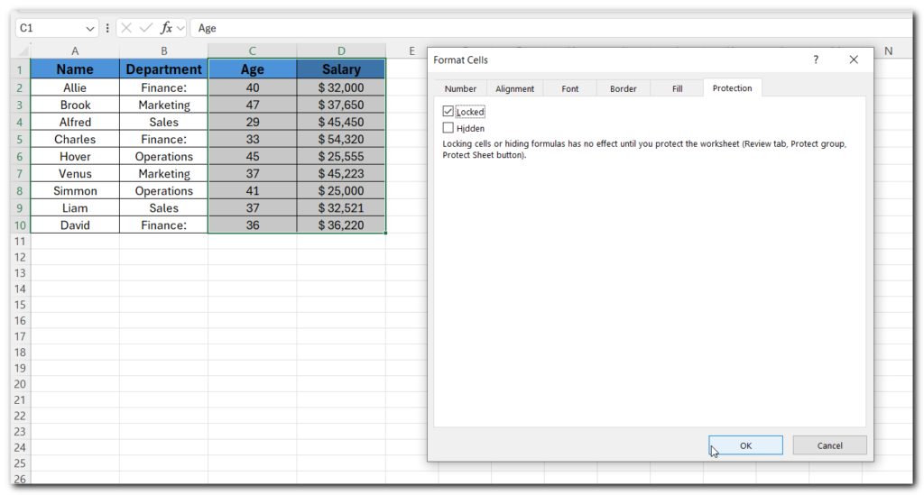
- Check the Locked box from the Protection tab.
- Click on OK.
- Go to the Review tab.
- From the Protect group, select Protect Worksheet.
- A “Protect Sheet” box will appear. Ensure the “Protect worksheet and contents of locked cells” option is checked.
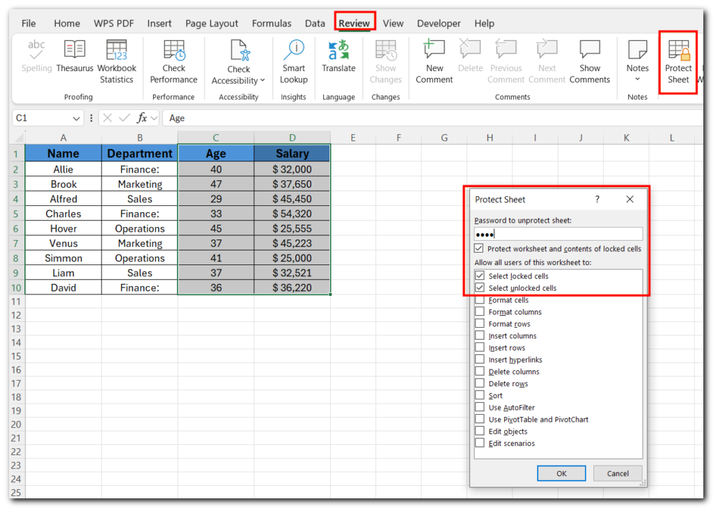
- Enter a password in the password field and click OK.
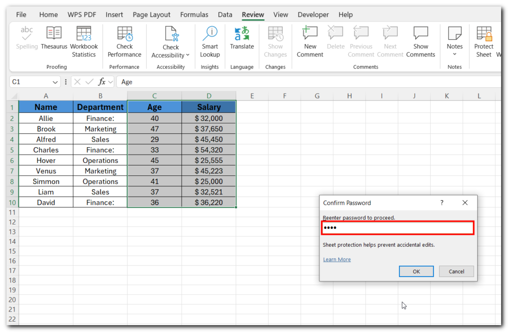
- If you entered a password in the previous box, a confirmation box will appear. Re-enter the password and click OK.
- once the selected columns are locked and the sheet is protected, a warning box will appear if anyone tries to edit those columns. The message will notify the user that the cells are protected and cannot be modified without the correct password.
Method 3:- Lock Column in Excel Using the ‘Allow Edit Ranges’ Feature
- Select the Review tab on the ribbon.
- In the Protect group, click Allow Edit Ranges.
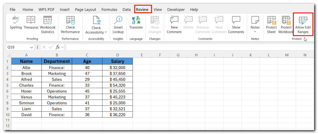
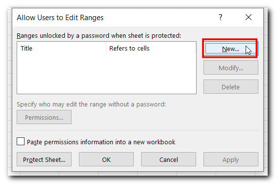
- In the dialog box that appears, click New to define a range of cells that users can edit.
- Select the range of cells that you want to allow editing.
- Set a password if desired (optional), and click OK.
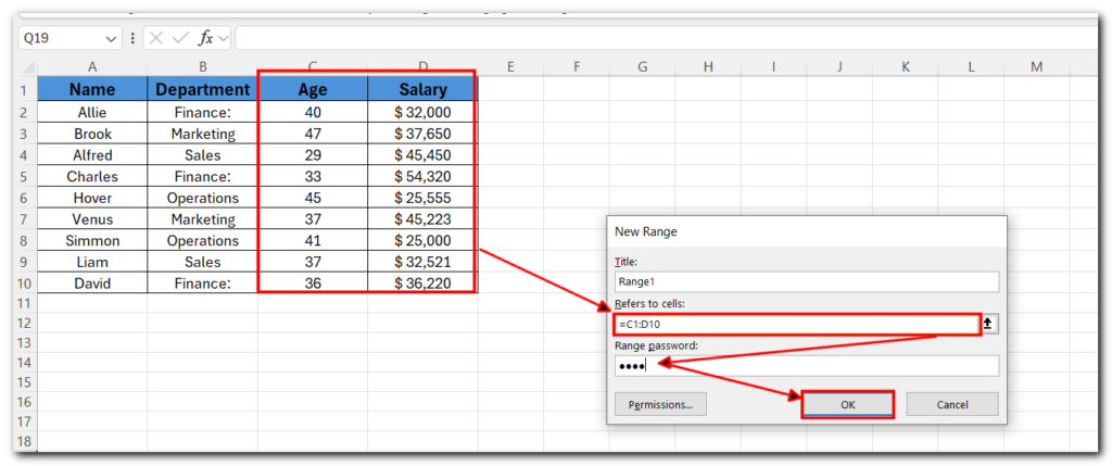
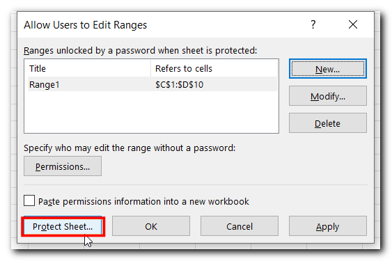
- In the Allow Users to Edit Ranges dialog box, select the range you’ve created.
- Click on Protect Sheet.
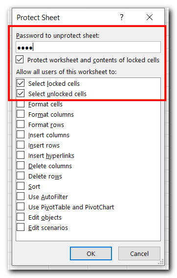
- In the Protect Sheet dialog, enter a password if you want to fully protect the sheet.
- Click OK.
- Now, only the specified ranges will be editable without a password, while the rest of the sheet will be locked.
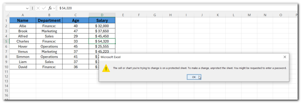
After completing all the steps, columns A and B will remain editable, while the rest of the cells, including columns C and D, will be protected from changes. If you try to edit any cell in columns C and D, a warning box will pop up, stopping you from making any changes unless you enter the correct password.
There are different way to Unhide Columns in Excel. To learn more about excel tips follow us now
Conclusion:-
And that’s how you can lock a column in Excel. You can use the same steps to lock rows, individual cells, or multiple columns, ensuring others can’t edit specific parts of your spreadsheet when sharing it.


