Hi Friends, we are starting with a new series of articles on a very important feature of MS Excel. Yes, that is Power Query. It was first introduced with Excel 2010 version and started gaining attention of users due to its capabilities and features. So, what is Power Query, let’s start from this question.
Through Power Query you can setup a query once and reuse it with a single click refresh button. As the businesses are growing so as the data is also increasing day by day. Power Query is a powerful feature which can import thousands and millions of records into the data model for analysis.
The user interface is also very intuitive and does not require special skill to learn it. With the easy navigation, you can quickly import your data and start analyzing in few minutes only.
So what you can do with your data through Power Query. Well the answer is Almost Everything. It allows multiple ways to import the data then transform it using cleanup, filters, sort etc. and finally Publish or export the data.
Using Power Query, you can import data from various source such as Excel, Text, Access, SQL, Web, Facebook, Azure and many more.
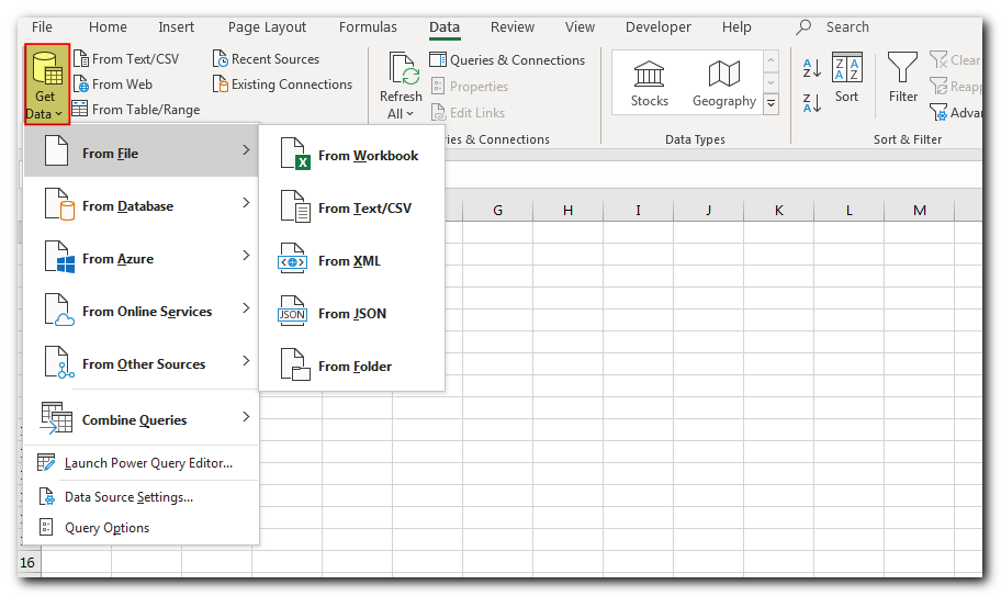
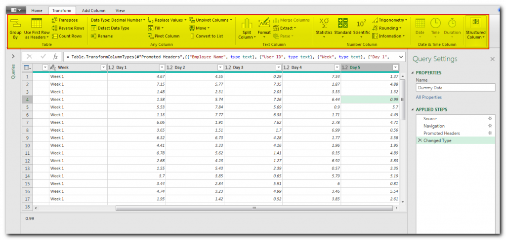
Once you have imported the data, the next step is to clean and transform it. You can do it through the amazing features provided by Power Query such as changing data types, removing columns rows, blanks, find and replace, text to column, split column, sum, rounding, calculations, filters, sort, transpose etc.
If you have multiple data sets that you want to consolidate into one query, then you can use append or merger queries feature.

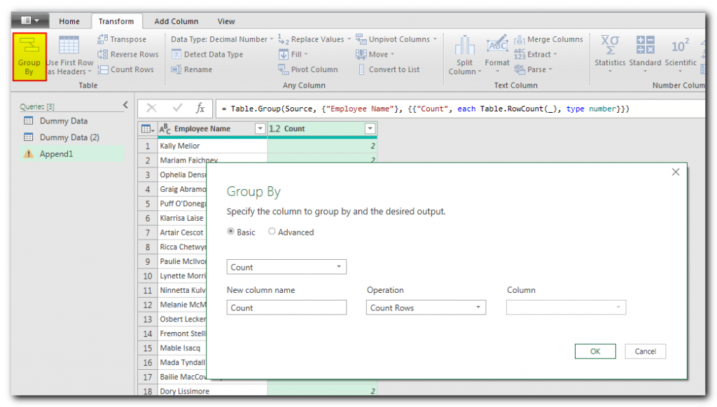
The next step is to summarize your data through Group By option.
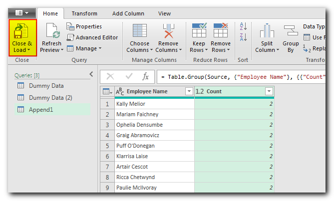
The final step is to publish or export your data to Excel file. You can do this through “Close & Load” button and your data is ready to share.
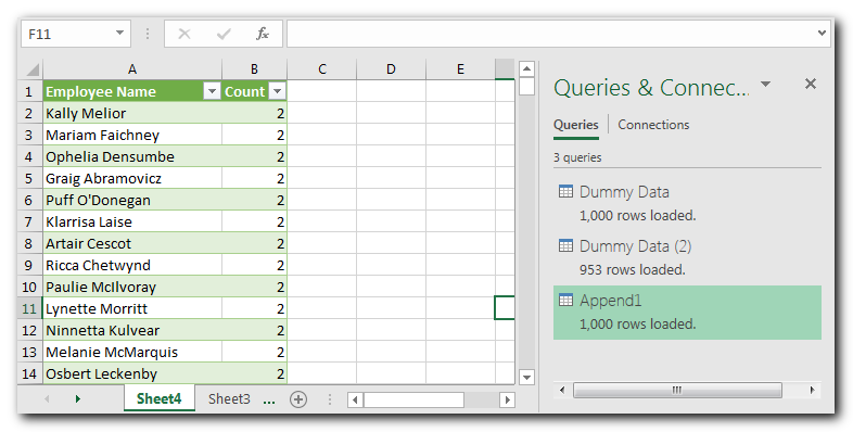
There are majorly two advantages of Power Queries as mentioned below

This tutorial shows how to use Goal Seek in Excel 365 – 2010 to get the result you want by changing an input value.
What-If Analysis is one of Excel’s most powerful but least understood features. Simply put, it lets you try out different scenarios and see possible outcomes. In other words, it helps you see how changes affect your data without actually changing the real data. In this tutorial, we’ll focus on one of Excel’s What-If Analysis tools—Goal Seek
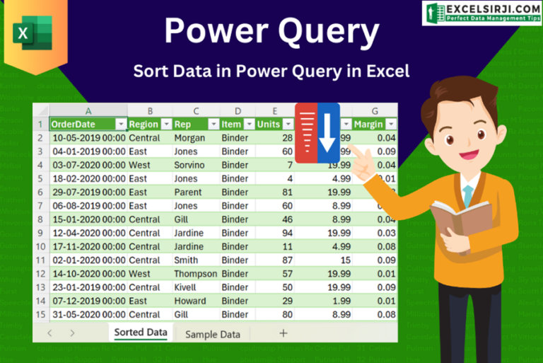
This article unveils the magic of Power Query, a built-in Excel tool that simplifies data organization. Learn how to sort by single or multiple columns, create layered sorts for complex needs, and even reverse your data order entirely. Power Query puts you in control, transforming your data into a well-structured format for effortless analysis.
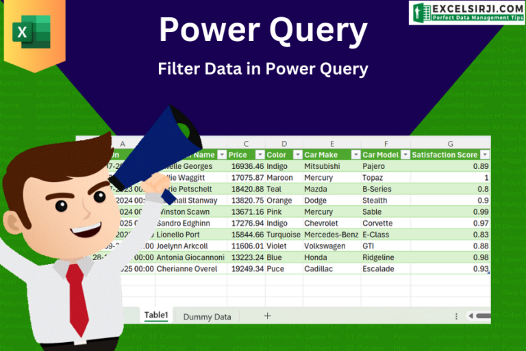
This step-by-step tutorial empowers you to leverage Power Query’s robust filtering capabilities. Learn to filter by date, text, numbers, and more, streamlining your workflow and unlocking deeper insights from your data. Watch now and elevate your Excel expertise!

This tutorial teaches the basics of correlation in Excel. It shows how to find a correlation coefficient, make a correlation matrix, and understand the results.
Correlation is one of the easiest calculations you can do in Excel. Even though it’s easy, it helps a lot in understanding how two or more things are related. Excel has all the tools you need to do a correlation analysis—you just need to know how to use them
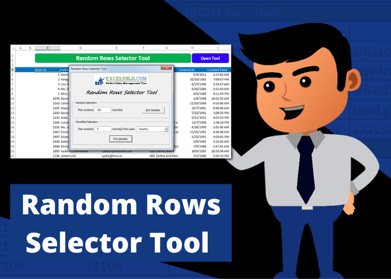
Random Rows Selector is an MS Excel based tool which can be used to pick random or stratified samples from a set of records available in Excel.
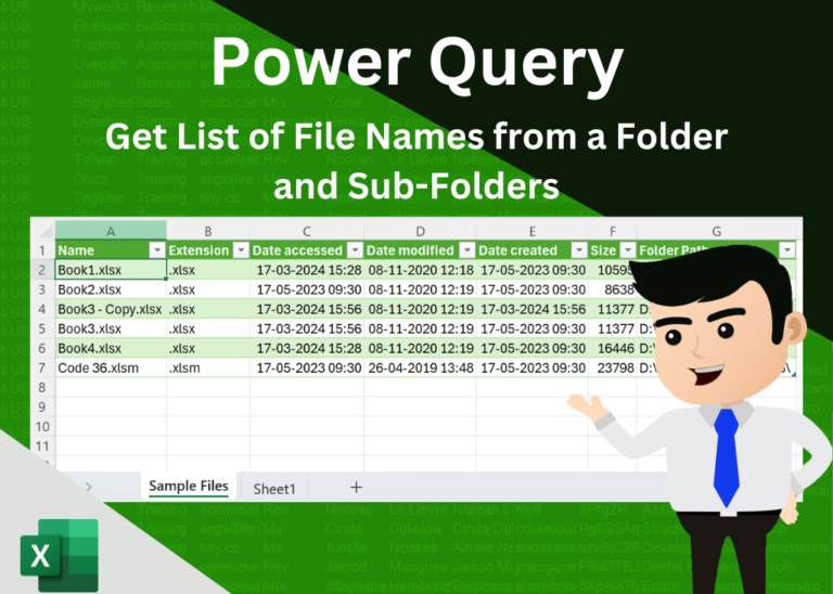
In today’s digital era, efficient file management is essential for productivity and organization. Whether you’re handling work documents or personal files, mastering effective file organization techniques can save you time and effort. In this step-by-step…
Very clear explanations.. Thanks.. Need more videos on PQ…