We have got many instances where we needed to generate a random database or values. “RAND function” is very useful for users who creates random database for various types of working and analysis.
“RAND Function” generates values between 0 to less than 1. We always have output of the “RAND function” in decimals. The formula of function is very simple because it has no arguments and provides the random output.
Syntax: =RAND()
Example: Suppose we need to create a database for the various types of stationery products and their prices for a month.
There is one way to mention the random product prices one by one or we can use the “RAND function” to make the work easy. Here we will go ahead with using function.
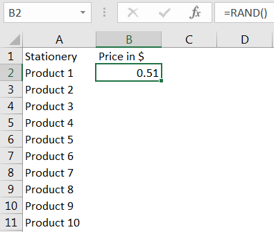
Drag the formula to respective cells. i.e. Select Column + Ctrl + D
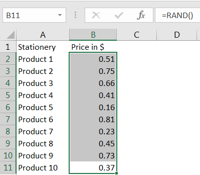
RANDBETWEEN Function is like the function “RAND” that we leant in above topic. RANDBETWEEN function is used where user needs integer values (not decimal) and between a predefined range.
Syntax: RANDBETWEEN(bottom, top)
Here, “bottom” means the lower value and “top” means higher value in range that you want
Example: You want to prepare a random database for volume of books in a books store with minimum quantity of 10 units and maximum quantity of 100 units. So here we need the various book name and random number of books.
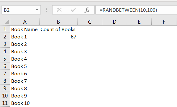
Drag the formula to respective cells. i.e. Select Column + Ctrl + D
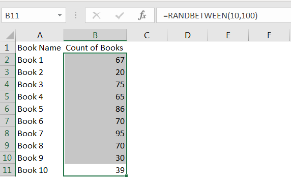
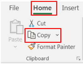
Select the data in column -> Menu- > Home-> Copy
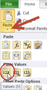
Go to -> Menu- > Home-> Paste Values
Please comment with your questions or feedback related to this article.
Want to learn more similar tricks? Please subscribe to us or follow us.
Keep Learning!!

This tutorial shows you how to change the row colors in Excel to automatically highlight every other row or every nth row or column in your worksheets. You will also learn how to use Excel’s banded rows and columns and find some helpful formulas to shade rows based on value changes.
Using alternating colors for rows in Excel is a common way to make data easier to read. While it’s simple to manually highlight rows in a small table, it can be very time-consuming in larger tables. A better approach is to automatically alternate the colors of rows or columns, and this article will show you how to do it quickly

RIGHT function is used for extracting the “Right Most” characters from the available string in Microsoft excel. Function returns value to new string.

Print Row Header on Each Page in Excel means that when you print your worksheet, the selected row (often the top row with column headers) will repeat at the top of every printed page. This ensures…

To subtract numbers in Excel, follow these steps:
Start by typing an equal sign (=) in the cell where you want the result.
Enter the first number or cell reference you want to subtract from.
Type a minus sign (-).
Enter the second number or cell reference you want to subtract.

This guide explains the basics of Excel’s Advanced Filter and shows you how to use it to find records that match one or more complicated conditions.
If you’ve read our previous guide, you know that Excel’s regular filter offers different options for filtering text, numbers, and dates. These options work well for many situations, but not all. When the regular filter isn’t enough, you can use the Advanced Filter to set up custom criteria that fit your exact needs.
Excel’s Advanced Filter is especially useful for finding data based on two or more complex conditions. For example, you can use it to find matches and differences between two columns, filter rows that match another list, or find exact matches with the same uppercase and lowercase letters.
Advanced Filter is available in all Excel versions from 365 to 2003. Click the links below to learn more.

LARGE function is used to get the Largest k-th value from the range.
LARGE Function has two required arguments i.e. array, and k