Excel Nested IF statement: examples, best practices and alternatives
This guide shows how to use the excel nested IF statement function in Excel to check several conditions. You will also learn about other functions that can be easier to use than a nested formula.
When you want to make decisions in Excel, you often use an IF formula. It checks if something is true, then gives one result if it is and another result if it isn’t. If you need to check more than one thing, you can put many IFs inside each other.
Although using multiple IFs is common, it’s not the only way to check several conditions in Excel. This guide will introduce you to some easier and useful alternatives.
Table of Contents
Excel nested IF statement
IF(condition1, result1, IF(condition2, result2, IF(condition3, result3, result4)))
You can see that each IF function is placed inside the value_if_false part of the previous IF function. Each IF has its own parentheses, but all the closing parentheses are grouped at the end of the formula.
Our example nested IF formula checks 3 conditions and gives 4 possible results (the 4th result is shown if none of the conditions are TRUE). In simple terms, this nested IF formula is telling Excel to do the following:
Test condition1, if TRUE – return result1, if FALSE –
test condition2, if TRUE – return result2, if FALSE –
test condition3, if TRUE – return result3, if FALSE –
return result4
As an example, let’s find out commissions for a number of sellers based on the amount of sales they’ve made:
Commission | Sales |
3% | $1 – $50 |
5% | $51 – $100 |
7% | $101 – $150 |
10% | Over $150 |
In math, changing the order of numbers you add doesn’t change the total. But in Excel, changing the order of IF functions changes the result. Why? Because a nested IF formula gives the result for the first condition that is TRUE. That’s why it’s important to arrange your conditions in the right order—either from high to low or low to high, depending on what you need. In our example, we check the ‘highest’ condition first, then the ‘next highest,’ and so on:
=IF(B2>150, 10%, IF(B2>=101, 7%, IF(B2>=51, 5%, IF(B2>=1, 3%, “”))))
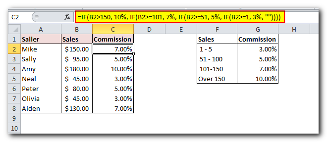
If we put the conditions in reverse order, from lowest to highest, the results would be wrong. The formula would stop after the first test (B2>=1) for any value greater than 1. For example, if we have $100 in sales, since it’s greater than 1, the formula wouldn’t check the other conditions and would return 3% as the answer.
If you prefer to arrange the conditions from low to high, use the ‘less than’ operator. Start by checking the ‘lowest’ condition first, then the ‘next lowest,’ and so on
=IF($B2<1, 0%, IF($B2<51, 3%, IF($B2<101, 5%, IF($B2<=150, 7%, 10%))))
As you can see, creating a nested IF formula that works correctly from start to finish requires a lot of careful thinking. While Excel lets you nest up to 64 IF functions in one formula, it’s not something you’d usually want to do. So, if you (or someone else) are staring at your nested IF formula, trying to understand what it does, it might be time to rethink your approach and consider using a different tool
Nested IF with OR/AND conditions
If you need to check several different sets of conditions, you can use the OR and AND functions. You can place these functions inside IF statements and then nest those IF statements inside each other
Nested IF in Excel with OR statements
By using the OR function, you can check two or more conditions in the IF function and return TRUE if any of them is TRUE. Let’s look at an example to see how it works.
Suppose you have two columns of sales—January sales in column B and February sales in column C. You want to check both columns and calculate the commission based on the higher number. Here’s the logic: if either January or February sales are more than $150, the seller gets a 10% commission. If either January or February sales are $101 or more, the seller gets a 7% commission, and so on.
To do this, write an OR statement like OR(B2>150, C2>150) and put it inside the IF function. This will create a formula like this:
=IF(OR(B2>150,
C2>150), 10%, IF(OR(B2>=101, C2>=101),7%, IF(OR(B2>=51, C2>=51),
5%, IF(OR(B2>=1, C2>=1), 3%, ""))))
And have the commission assigned based on the higher sales amount:

Nested IF in Excel with AND statements
If your tests involve more than one condition, and all of them need to be TRUE, use the AND function.
For example, to calculate commissions based on the lower number of sales, take the same formula as above but replace OR with AND. In other words, you tell Excel to give 10% commission only if both January and February sales are more than $150, and 7% if both January and February sales are $101 or more, and so on
=IF(AND(B2>150, C2>150), 10%, IF(AND(B2>=101, C2>=101), 7%, IF(AND(B2>=51, C2>=51), 5%, IF(AND(B2>=1, C2>=1), 3%, “”))))
As the result, our nested IF formula calculates the commission based on the lower number in columns B and C. If either column is empty, there is no commission at all because none of the AND conditions is met:

If you’d like to return 0% instead of blank cells, replace an empty string (””) in the last argument with 0%:
=IF(AND(B2>150,C2>150), 10%, IF(AND(B2>=101, C2>=101), 7%, IF(AND(B2>=51,C2>=51), 5%,IF(AND(B2>=1, C2>=1), 3%, 0%))))

VLOOKUP instead of nested IF in Excel
When working with ‘scales,’ or continuous ranges of numbers that cover the entire range, you can often use the VLOOKUP function instead of nested IFs.
First, create a reference table like the one shown in the screenshot. Then, write a VLOOKUP formula using an approximate match, which means setting the range_lookup argument to TRUE.
Assuming the lookup value is in B2 and the reference table is F2:G5, the formula goes as follows:
=VLOOKUP(B2,$F$2:$G$5,2,TRUE)
Please notice that we fix the table_array with absolute references ($F$2:$G$5) for the formula to copy correctly to other cells:
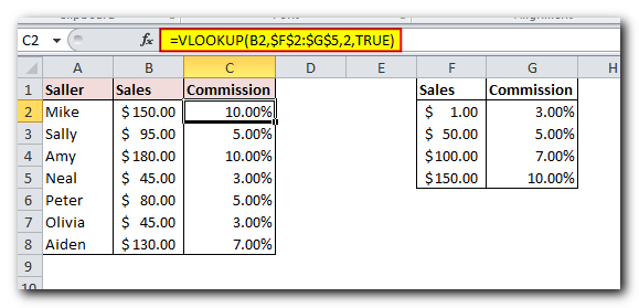
When you set the last part of your VLOOKUP formula to TRUE, you tell Excel to find the closest match. If it doesn’t find an exact match, it will return the next largest value that is smaller than the number you’re looking for. This way, your formula will work for exact values as well as numbers that fall in between.
For example, if the lookup value in B3 is $95, this number isn’t in the lookup table. A VLOOKUP with exact match would give an #N/A error. But with approximate match, it keeps looking until it finds the nearest value smaller than $95 (which is $50), and returns a value from the second column (which is 5%).
However, if the lookup value is smaller than the smallest number in the table, or if the lookup cell is empty, the formula will return an #N/A error. If you want to avoid this, you can nest VLOOKUP inside IFERROR and tell Excel what to show when the lookup value isn’t found. For example
=IFERROR(VLOOKUP(B2, $F$2:$G$5, 2, TRUE), “Outside range”)
Important note! For a Vlookup formula with approximate match to work correctly, the first column in the lookup table must be sorted in ascending order, from smallest to largest.
IFS statement as alternative to nested IF function
In Excel 2016 and later versions, Microsoft introduced a special function to evaluate multiple conditions – the IFS function.
An IFS formula can handle up to 127 logical_test/value_if_true pairs, and the first logical test that evaluates to TRUE “wins”:
IFS(logical_test1, value_if_true1, [logical_test2, value_if_true2]…)
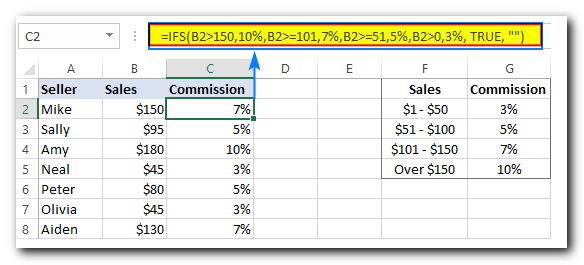
In accordance with the above syntax, our nested IF formula can be reconstructed in this way:
=IFS(B2>150, 10%, B2>=101, 7%, B2>=51, 5%, B2>0, 3%)
Be aware that the IFS function gives an #N/A error if none of the conditions you set are met. To prevent this, you can add one more logical_test/value_if_true at the end of your formula. This will return 0, an empty string (“”), or any other value you choose if none of the earlier tests are TRUE.
=IFS(B2>150, 10%, B2>=101, 7%, B2>=51, 5%, B2>0, 3%, TRUE, “”)
As the result, our formula will return an empty string (blank cell) instead of the #N/A error if a corresponding cell in column B is empty or contains text or negative number.
Note. Like nested IF, Excel’s IFS function returns a value corresponding to the first condition that evaluates to TRUE, which is why the order of logical tests in an IFS formula matters.
CHOOSE instead of nested IF formula in Excel
Another way to test multiple conditions within a single formula in Excel is using the CHOOSE function, which is designed to return a value from the list based on a position of that value.
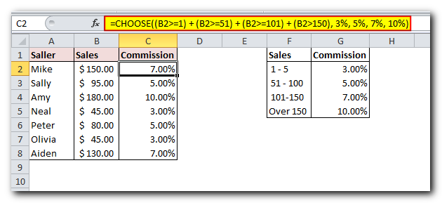
Applied to our sample dataset, the formula takes the following shape:
=CHOOSE((B2>=1)+ (B2>=51) + (B2>=101) + (B2>150), 3%, 5%, 7%, 10%)
In the first argument (index_num), you check all the conditions and add up the results. Since TRUE counts as 1 and FALSE counts as 0, this helps you find the position of the value to return.
For example, if the value in B2 is $150, the first three conditions are TRUE, and the last one (B2 > 150) is FALSE. This means index_num equals 3, so the formula returns the 3rd value, which is 7%
Tip. If none of the logical tests is TRUE, index_num is equal to 0, and the formula returns the #VALUE! error. An easy fix is wrapping CHOOSE in the IFERROR function like this:
=IFERROR(CHOOSE((B2>=1) + (B2>=51) + (B2>=101) + (B2>150), 3%, 5%, 7%, 10%), “”)
SWITCH function as a concise form of nested IF in Excel
When you have a fixed set of specific values instead of ranges, the SWITCH function can be a simpler option than using complex nested IF statements
SWITCH(expression, value1, result1, value2, result2, …, [default])
The SWITCH function checks an expression against a list of values and returns the result for the first match it finds.
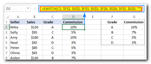
If you want to calculate the commission based on grades instead of sales amounts, you can use this simpler version of a nested IF formula in Excel
=SWITCH(C2, “A”, 10%, “B”, 7%, “C”, 5%, “D”, 3%, “”)
Or, you can make a reference table like shown in the screenshot below and use cell references instead of hardcoded values:
=SWITCH(C2, $F$2, $G$2, $F$3, $G$3, $F$4, $G$4, $F$5, $G$5, “”)
Please notice that we lock all references except the first one with the $ sign to prevent them from changing when copying the formula to other cells
Note. The SWITCH function is only available in Excel 2016 and higher.
Concatenating multiple IF functions in Excel
As mentioned before, the SWITCH function was introduced in Excel 2016. If you’re using an older version of Excel and want to do something similar, you can combine two or more IF statements using the concatenate operator (&) or the CONCATENATE function.
For example:
=(IF(C2=”a”, 10%, “”) & IF(C2=”b”, 7%, “”) & IF(C2=”c”, 5%, “”) & IF(C2=”d”, 3%, “”))*1
Or
=CONCATENATE(IF(C2=”a”, 10%, “”), IF(C2=”b”, 7%, “”), IF(C2=”c”, 5%, “”) & IF(C2=”d”, 3%, “”))*1
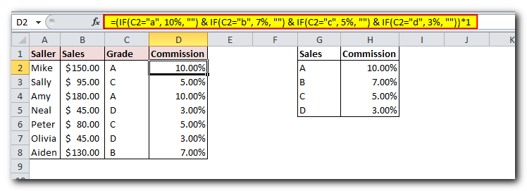
As you may have noticed, we multiply the result by 1 in both formulas. This is done to change the text returned by the CONCATENATE formula into a number. If you want your output to be text, you don’t need to multiply.
For more information, check out the CONCATENATE function in Excel
You can see that Microsoft Excel offers several good alternatives to nested IF formulas. I hope this tutorial has given you some ideas on how to use them in your worksheets. If you want to take a closer look at the examples from this tutorial, feel free to download our sample workbook below. Thank you for reading, and I hope to see you on our blog next week


