Excel named range – how to define and use names in Excel
This tutorial explains what an Excel name is and shows you how to define a name for a cell, range, constant, or formula. You’ll also learn how to edit, filter, and delete defined names in Excel.
Excel names are a bit of a paradox: they’re one of the most useful features, but many people find them unnecessary or too technical. That’s because few users truly understand what Excel names can do. This tutorial will not only teach you how to create a named range in Excel but also show you how this feature can make your formulas easier to write, read, and reuse.
Table of Contents
What does name mean in Excel?
In everyday life, we use names to refer to people, places, and things. For example, instead of saying “the city at latitude 40.7128° N and longitude 74.0059° W,” you just say “New York City.”
In Microsoft Excel, you can do something similar by giving a readable name to a single cell or a range of cells, allowing you to refer to them by name instead of their cell reference.
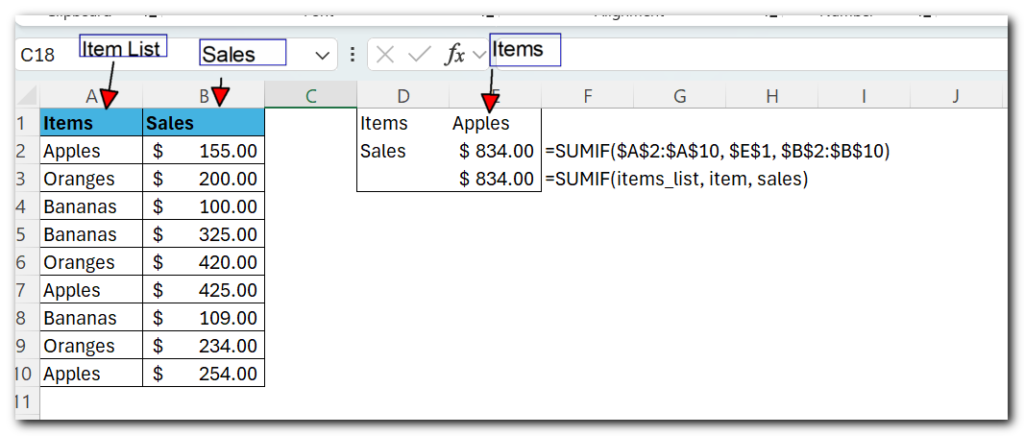
For instance, to find the total of sales (B2:B10) for a specific item (E1), you can use the following formula:
=SUMIF($A$2:$A$10, $E$1, $B$2:$B$10)
Or, you can give meaningful names to the ranges and individual cells and supply those names to the formula:
=SUMIF(items_list, item, sales)
Looking at the screenshot below, which of the two formulas are easier for you to understand?
Excel name types
In Microsoft Excel, there are two types of names you can create and use:
- **Defined name**: This is a name you assign to a single cell, range of cells, constant value, or formula. For example, when you name a range of cells, it’s called a named range or defined range. This tutorial focuses on these names.
2. **Table name**: This is the name given to an Excel table automatically when you create a table in a worksheet (using Ctrl + T). For more on Excel tables, check out How to make and use a table in Excel.
How to create an Excel named range
Overall, there are 3 ways to define a name in Excel: Name Box, Define Name button, and Excel Name Manager.
Type a name in the Name Box
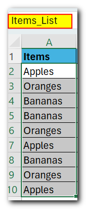
The Name Box in Excel is fastest way to create a named range:
- Select a cell or a range of cells that you want to name.
- Type a name into the Name Box.
- Press the Enter key.
Great, a new Excel named range is created!
Create a name by using the Define Name option
Another way to make a named range in Excel is this:
- Select the cell(s).
- On the Formulas tab, in the Define Names group, click the Define Name button.
- In the New Name dialog box, specify three things:
- In the Name box, type the range name.
- In the Scope dropdown, set the Name Scope (Workbook by default).
- In the Refers to box, check the reference and correct it if needed.
- Click OK to save the changes and close the dialog box.
Note: By default, Excel creates a name with absolute references. If you want a relative named range instead, just remove the $ sign from the reference. Before doing this, make sure you understand how relative names work in worksheets
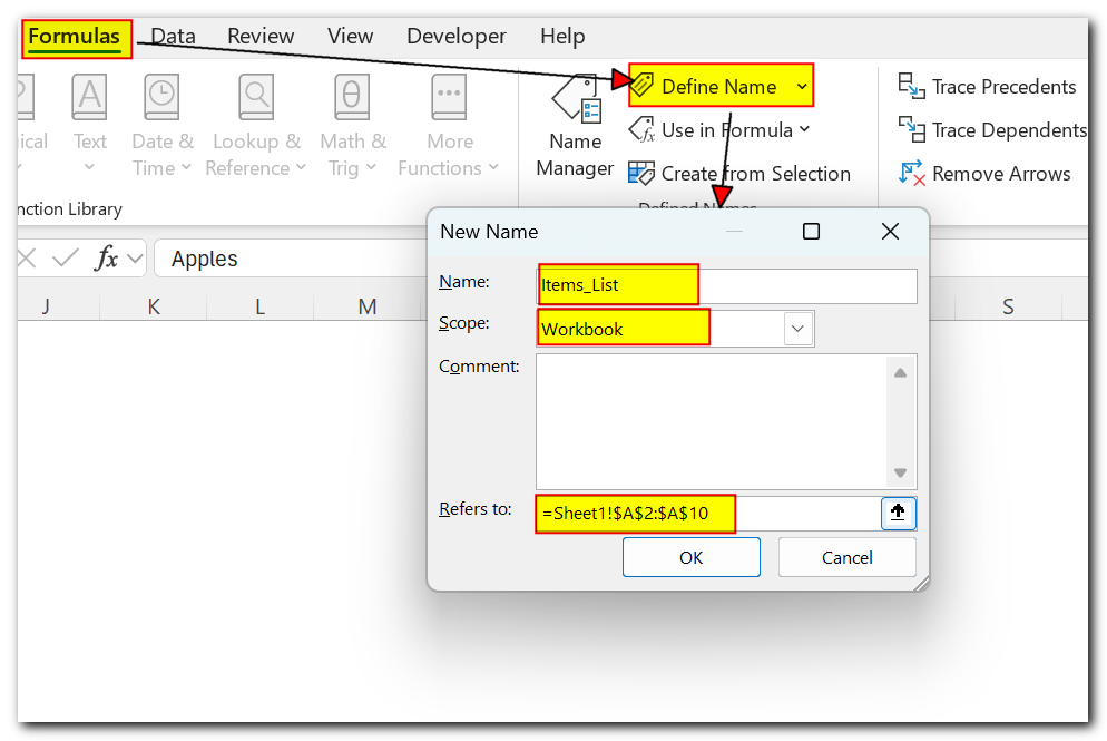
Using the Define Name option in Excel takes a few more clicks than the previous method, but it offers extra features like setting the name’s scope and adding a comment to explain the name. Plus, with Define Name, you can create a name for a constant or a formula.
Make a named range by using Excel Name Manager
Typically, the Name Manager in Excel is used to manage existing names, but you can also use it to create a new name. Here’s how:
- Go to the Formulas tab, then click on Name Manager in the Defined Names group. Or, simply press Ctrl + F3 (which is quicker and my preferred method).
- In the Name Manager window, click the New… button in the top left corner:
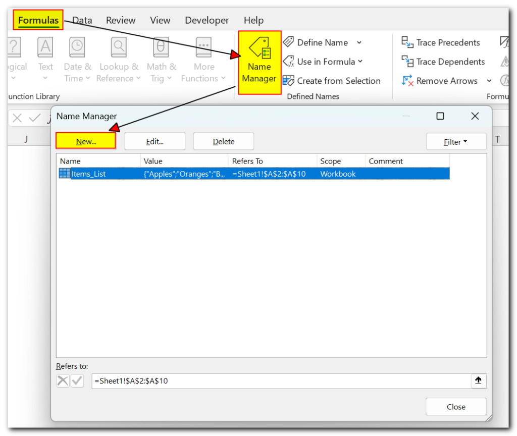
3.This will open the New Name dialog box where you configure a name as demonstrated in the previous section.
How to create an Excel name for a constant
In addition to named ranges, Excel lets you create a name without a cell reference that acts like a constant. You can do this using the Define Name feature or Name Manager as explained earlier.
For example, you can create a name like USD_EUR (for the USD to EUR conversion rate) and assign it a fixed value. Just type the value with an equal sign (=) in the Refers to field, like this: =0.93
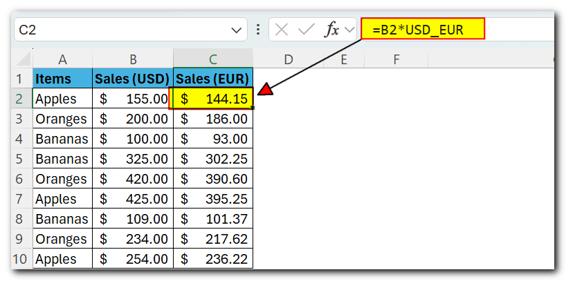
As soon as the exchange rate changes, you update the value only in one central location, and all your formulas will get recalculated in a single step!
How to define a name for a formula
In a similar manner, you can give a name to an Excel formula, for example, the one that returns the count of non-empty cells in column A, excluding the header row (-1):
=COUNTA(Sheet5!$A:$A)-1
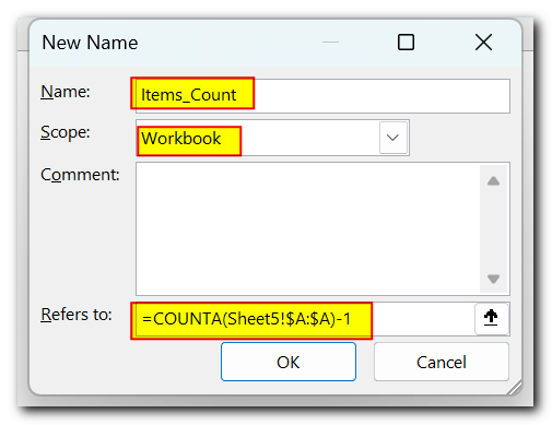
Note – If your formula refers to any cells on the current sheet, you do not need to include the sheet name in the references, Excel will do it for you automatically. If you are referencing a cell or range on another worksheet, add the sheet’s name followed by the exclamation point before the cell/range reference (like in the formula example above).
Now, whenever you want to know how many items there are in column A on Sheet5, not including the column header, just type the equality sign followed by the name of your formula in any cell, like this: =Items_count
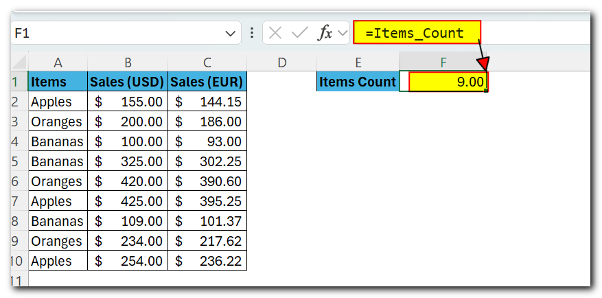
How to name columns in Excel (names from selection)
If your data is arranged in a tabular form, you can quickly create names for each column and/or row based on their labels:
- Select the entire table including the column and row headers.
- Go to the Formulas tab > Define Names group, and click the Create from Selection button. Or, press the keyboard shortcut Ctrl + Shift + F3.
- Either way, the Create Names from Selection dialogue box will open. You select the column or row with headers, or both, and click OK.
In this example, we have headers in the top row and left column, so we select these two options:
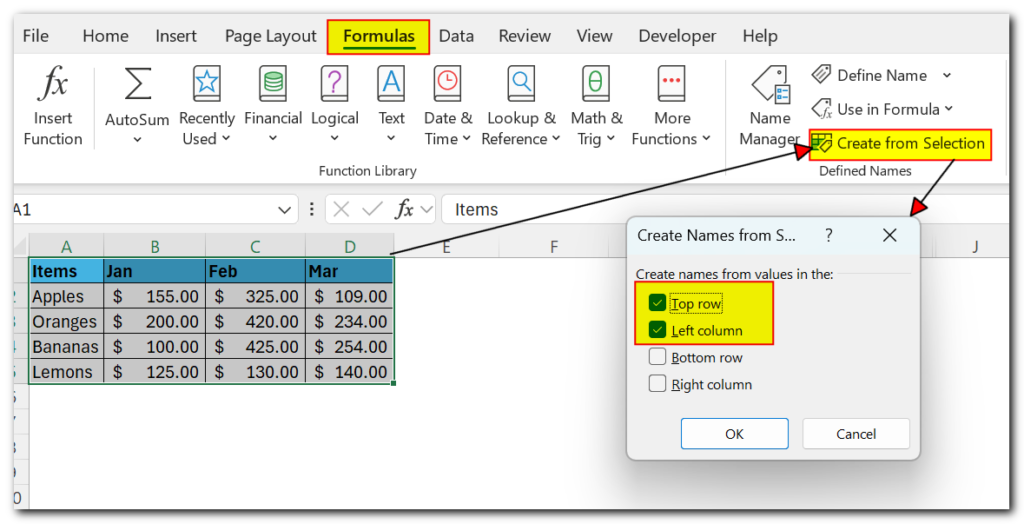
As the result, Excel will create 7 named ranges, picking up names from the headers automatically:
- Apples, Bananas, Lemons and Oranges for rows, and
- Jan, Feb and Mar for columns.

Excel naming rules
When creating a name in Excel, keep these rules in mind:
- An Excel name should be less than 255 characters long.
- Names cannot contain spaces or most punctuation marks.
- A name must start with a letter, underscore (_), or backslash (). If it starts with anything else, Excel will show an error.
- Excel names are case-insensitive, so “Apples”, “apples”, and “APPLES” are treated as the same name.
- You can’t name a range the same as a cell reference, like “A1” or “AA1”.
- You can use a single letter to name a range, like “a”, “b”, or “D”, except for “r”, “R”, “c”, and “C” (these letters are used as shortcuts for selecting a row or column when typed in the NameBox).
Excel Name Manager - quick way to edit, delete and filter names
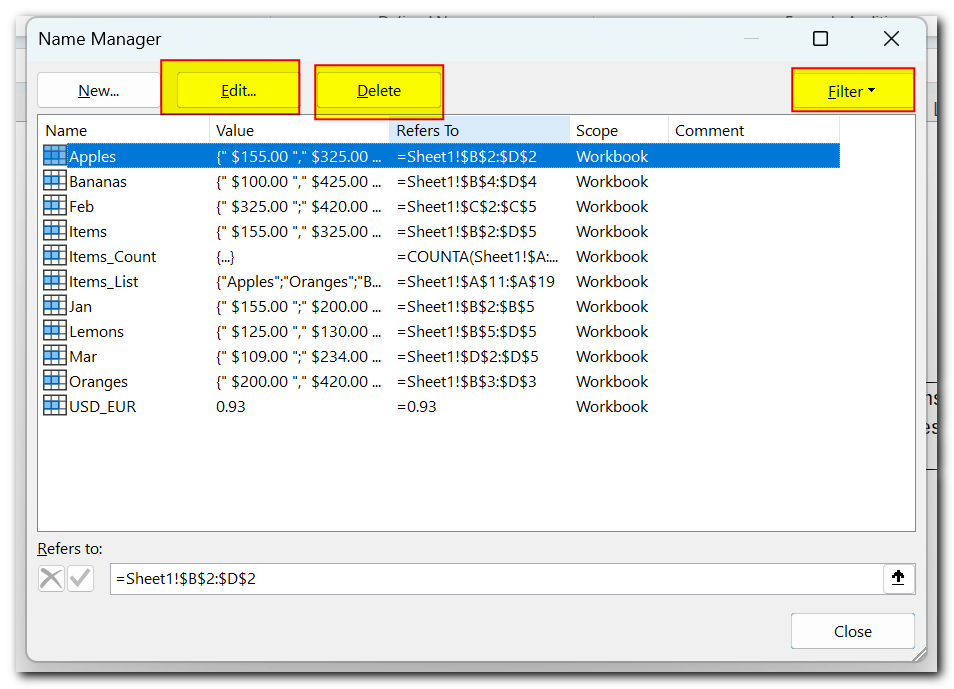
As its name suggests, the Excel Name Manager is specially designed to manage names: change, filter, or delete existing names as well as create new ones.
There are two ways to get to the Name Manager in Excel:
- On the Formulas tab, in the Define Names group, click the Name Manager

Press the Ctrl + F3 shortcut.
This will open the Name Manager window, where you can see all the names in the current workbook. From there, you can select the name you want to work with and use one of the three buttons at the top to edit, delete, or filter the name.
How to edit named range in Excel
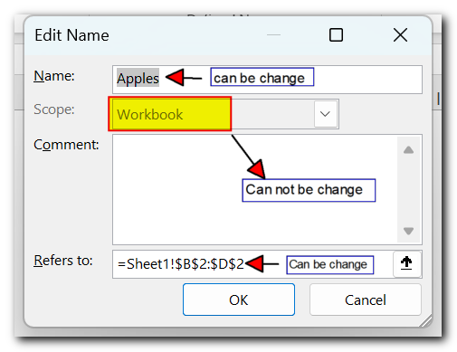
To change an existing name in Excel, open the Name Manager, select the name, and click the Edit… button. This will open a dialog box where you can update the name and reference. However, you can’t change the scope of the name
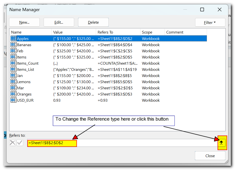
To edit a name’s reference, you don’t need to open the Edit
Name dialog box. Simply select the name in the Excel Name Manager, then type a
new reference directly in the ‘Refers to’ box or click the button on the right
to select a new range on the sheet. After you click Close, Excel will ask if
you want to save the changes—just click Yes
How to filter names in Excel
If you have many names in a workbook, you can click the Filter button at the top right corner of the Excel Name Manager window to see only the names that are relevant now. You can filter by:
- Names scoped to a worksheet or workbook
- Names with or without errors
- Defined names or table names
How to delete named range in Excel
To delete a named range, select it in the Name Manager and click the Delete button at the top.
To delete multiple names, click the first name, hold the Ctrl key, and click the other names you want to remove. Then, click Delete to remove all the selected names at once.
To delete all defined names in a workbook, click the first name, hold the Shift key, then click the last name. Release the Shift key and click Delete.
How to delete defined names with errors
If you have a number of invalid names with reference error, click the Filter button > Names with Errors to filter them:
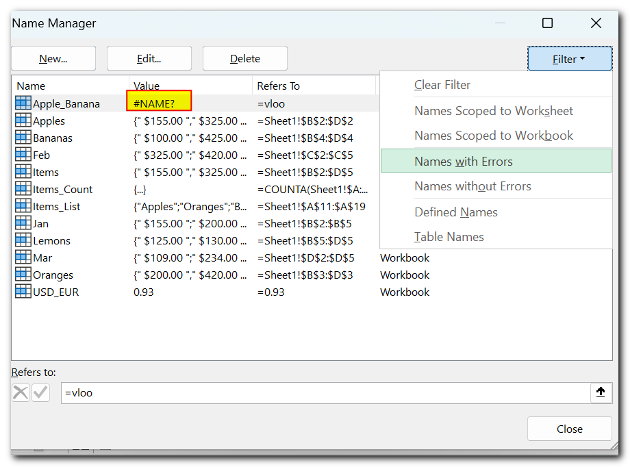
After that, select all filtered names as explained above (by using the Shift key), and click the Delete button.
Top 5 benefits of using names in Excel
So far in this tutorial, we’ve focused on how to create, and use named ranges in Excel. But you might be wondering, what makes Excel names so special and worth the effort? Here are the top five advantages of using defined names in Excel
1. Excel names make formulas easier to make and read
You don’t need to type complex references or keep selecting ranges on the sheet. Just start typing the name you want to use in the formula, and Excel will show a list of matching names. Double-click the name you want, and Excel will insert it into the formula right away

2. Excel names allow creating expandable formulas
By using dynamic named ranges, you can create a formula that automatically includes new data in calculations, so you don’t have to update every reference manually
3. Excel names make formulas easier to re-use
Excel names make it a lot easier to copy a formula to another sheet or port a formula into a different workbook. All you have to do is create the same names in the destination workbook, copy/paste the formula as is, and you will get it working immediately.
4. Named ranges simplify navigation
To quickly get to a specific named range, just click on its name in the Name box. If a named range resides on another sheet, Excel will take you to that sheet automatically.
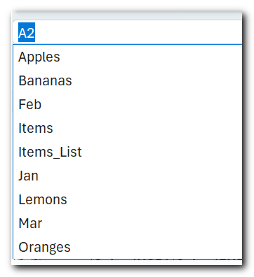
5. Named ranges allow creating dynamic drop-down lists
To create a drop-down list that expands and updates automatically, first make a dynamic named range, then create a data validation list based on that range. You can find detailed step-by-step instructions here: How to create a dynamic dropdown in Excel
This is how you create and use names in Excel. I thank you for reading and hope to see you on our blog next week!


