Similar Posts

EXCEL FUNCTION – REPT
REPT function is used to repeat the text or cell reference to multiple times

EXCEL FUNCTION – COUNTIF
Excel Function COUNTIF COUNTIF Excel Function is also one of the most used function in excel. This helps the user to calculate the number of counts based on single logic given by the user. You…

Calculate and highlight 90/60/30 days from or before today in Excel
The tutorial demonstrates how to find a date any number of days before or after today, counting either all days or only business days.
EXCEL FUNCTION – RAND
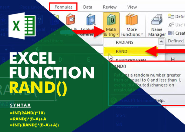
Generate Random Numbers in Excel Using RAND We have got many instances where we needed to generate a random database or values. Rand function is very useful for the users who creates random database for…

EXCEL FUNCTION – NETWORKDAYS
“NETWORKDAYS” function is very helpful feature in the Microsoft excel to calculate the working days from a particular period excluding “Saturday and Sundays”. NETWORKDAYS function subtract the Start Day from the End Date provided.
Practice EOMONTH & EDATE Function Online in Excel
Watch: How to use EOMONTH & EDATE Function in Excel? What is EOMONTH Function? The EOMONTH function in Excel returns the last day of a month based on a given date and a specified number of…

EXCEL FUNCTION – REPT
REPT function is used to repeat the text or cell reference to multiple times

EXCEL FUNCTION – COUNTIF
Excel Function COUNTIF COUNTIF Excel Function is also one of the most used function in excel. This helps the user to calculate the number of counts based on single logic given by the user. You…

Calculate and highlight 90/60/30 days from or before today in Excel
The tutorial demonstrates how to find a date any number of days before or after today, counting either all days or only business days.

EXCEL FUNCTION – RAND
Generate Random Numbers in Excel Using RAND We have got many instances where we needed to generate a random database or values. Rand function is very useful for the users who creates random database for…

EXCEL FUNCTION – NETWORKDAYS
“NETWORKDAYS” function is very helpful feature in the Microsoft excel to calculate the working days from a particular period excluding “Saturday and Sundays”. NETWORKDAYS function subtract the Start Day from the End Date provided.

Practice EOMONTH & EDATE Function Online in Excel
Watch: How to use EOMONTH & EDATE Function in Excel? What is EOMONTH Function? The EOMONTH function in Excel returns the last day of a month based on a given date and a specified number of…

EXCEL FUNCTION – REPT
REPT function is used to repeat the text or cell reference to multiple times

EXCEL FUNCTION – COUNTIF
Excel Function COUNTIF COUNTIF Excel Function is also one of the most used function in excel. This helps the user to calculate the number of counts based on single logic given by the user. You…

Calculate and highlight 90/60/30 days from or before today in Excel
The tutorial demonstrates how to find a date any number of days before or after today, counting either all days or only business days.

EXCEL FUNCTION – RAND
Generate Random Numbers in Excel Using RAND We have got many instances where we needed to generate a random database or values. Rand function is very useful for the users who creates random database for…

EXCEL FUNCTION – NETWORKDAYS
“NETWORKDAYS” function is very helpful feature in the Microsoft excel to calculate the working days from a particular period excluding “Saturday and Sundays”. NETWORKDAYS function subtract the Start Day from the End Date provided.

Practice EOMONTH & EDATE Function Online in Excel
Watch: How to use EOMONTH & EDATE Function in Excel? What is EOMONTH Function? The EOMONTH function in Excel returns the last day of a month based on a given date and a specified number of…


