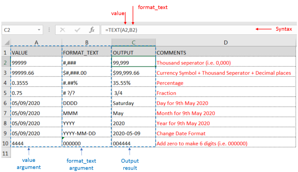
=TEXT(value,format_text)
value argument [Required] is used to give the text or cell reference for which formatting is to be changed
format_text [Required], is used to give the formatting code as per the requirement
Here we have some examples, where “Column A” has various values, “Column B” represents format_text and “Column C” shows the output of the function.
We will be using TEXT function as follows:

– Format of cell can also be changed by following CTRL+1 (or MAC Command button +1) and select the desired format/appearance
– If cell reference is not correctly provided in the function, then it will give output as an error
– Function should give output in “General” format, however if output is not as per the desired format then we need to change the cell format to “GENERAL”
Hope you learnt this Function,
Don’t forget to leave your valuable comments!
If you liked this article and want to learn more similar tricks, please Subscribe us or follow us on Social Media by clicking below buttons:

SMALL function is used to get the Smallest k-th value from the range.
SMALL Function has two required arguments i.e. array, and k

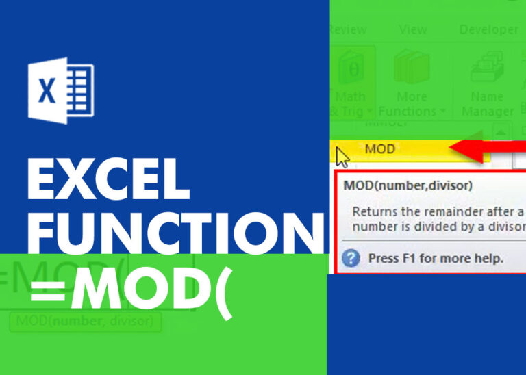
MOD function is used to get the remainder of number that is divided by divisor. MOD Function has two required arguments i.e. number and divisor.

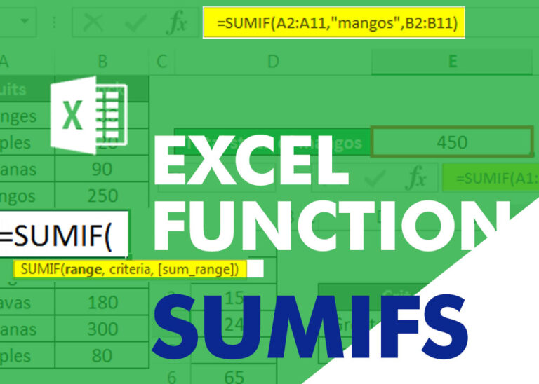
SUMIFS function is used to get the “total sum” of values for matching criteria across range. SUMIFS Function has required and optional arguments

Watch: How to use VLOOKUP Function in Excel? What is VLOOKUP Function? The VLOOKUP function in Excel searches for a value in a table and returns a corresponding value from another column in the same row…

Watch Video: Rand and Randbetween Excel Functions Generate Random Numbers using Excel Functions We have got many instances where we needed to generate a random database or values. “RAND function” is very useful for users…

Excel Function- WORKDAY.INTL WORKDAY.INTL function is an advanced version of WORKDAY function with additional advantage of “Custom weekend options” For Example, with WORKDAY function weekends are treated as “Saturday and Sundays” however if you need…