Excel Function SUMIFS is used to get the “total sum” of values for matching criteria across range.
SUMIFS Function is used to get total sum with more than one criteria. It has required arguments i.e. sum_range, criteria_range1, criteria1 and Optional arguments i.e. [criteria_range2, criteria2]… We can place add more than one range to include multiple criteria or conditions.
SUMIFS function is used to get the “total sum” of values for matching criteria across range.
SUMIFS Function has required arguments i.e. sum_range, criteria_range1, criteria1 and Optional arguments i.e. [criteria_range2, criteria2]… We can place add more than one range to include multiple criteria or conditions.
The syntax is as follows:
SUMIF(range, criteria, [sum_range])
sum_range argument is used to give cell range; those are to be added together as per the criteria mentioned below
criteria_range1 argument is used to give the range in which criteria1 needs to find
criteria1 argument is used to give criteria for sum. We can give value (example “A”, >10, 50) or cell reference# (example: E2) in this argument
[criteria_range2] optional argument is used to give the ANOTHER range in which criteria2 needs to find
[criteria2] optional argument is used to give criteria2 for sum. Value or cell reference# can be given.
Kindly note, we can add multiple criteria in the function by separating them with Comma (,)
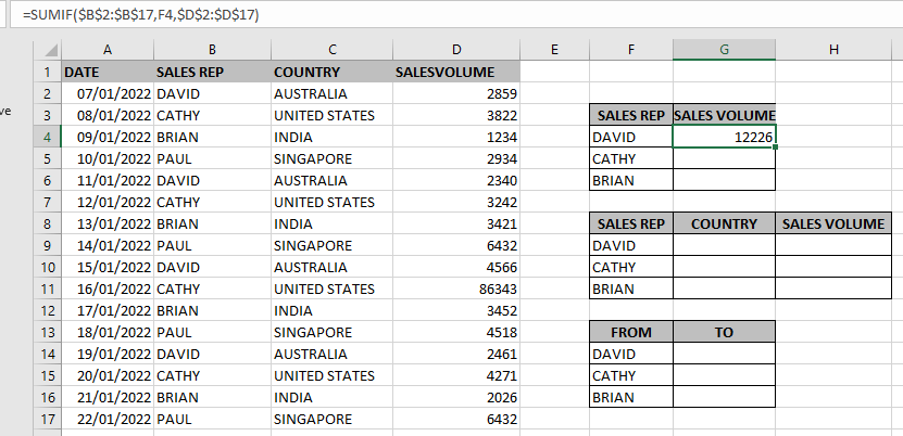
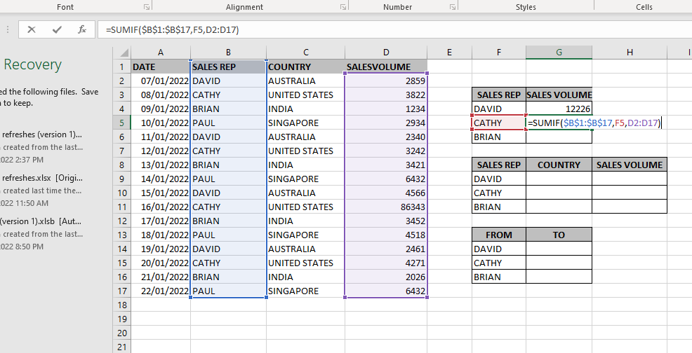
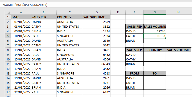
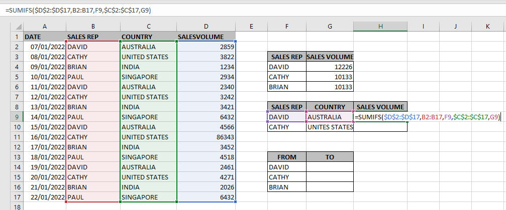
We will be using SUMIF function as follows:
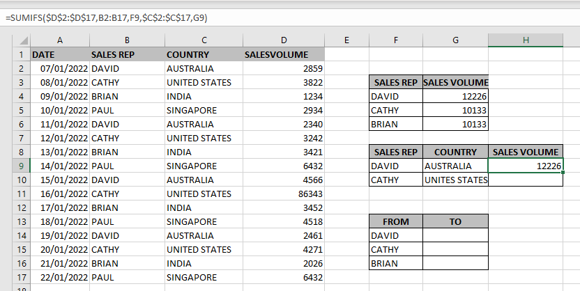
Hope you learnt this Function,
Don’t forget to leave your valuable comments!
If you liked this article and want to learn more similar tricks, please Subscribe us.

FIND function is used to find the position of text, or character in an available string.

INDIRECT function is used to convert the text/string into cell reference. Function provides output as the value of that cell reference.

This tutorial explains what an Excel name is and shows you how to define a name for a cell, range, constant, or formula. You’ll also learn how to edit, filter, and delete defined names in Excel.
Excel names are a bit of a paradox: they’re one of the most useful features, but many people find them unnecessary or too technical. That’s because few users truly understand what Excel names can do. This tutorial will not only teach you how to create a named range in Excel but also show you how this feature can make your formulas easier to write, read, and reuse.
Blank rows in Excel can be a real hassle, making it harder to move around and work with your data. But don’t worry—there are plenty of easy ways to get rid of these unwanted rows….

COUNT function is used to get the total count of Number values in range or list.COUNT Function has one required and optional arguments.

This guide explains the basics of Excel’s Advanced Filter and shows you how to use it to find records that match one or more complicated conditions.
If you’ve read our previous guide, you know that Excel’s regular filter offers different options for filtering text, numbers, and dates. These options work well for many situations, but not all. When the regular filter isn’t enough, you can use the Advanced Filter to set up custom criteria that fit your exact needs.
Excel’s Advanced Filter is especially useful for finding data based on two or more complex conditions. For example, you can use it to find matches and differences between two columns, filter rows that match another list, or find exact matches with the same uppercase and lowercase letters.
Advanced Filter is available in all Excel versions from 365 to 2003. Click the links below to learn more.