Watch Excel Tutorial Video – Excel Function – SUMIF

How to use SUMIF function in Excel?

Complete Excel VBA Course

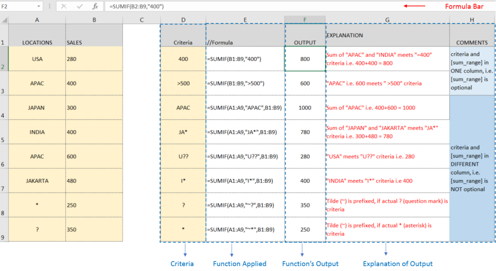
SUMIF function is used to get the “total sum” of values for matching criteria across range.

SUMIF Function has two required arguments i.e. rangecriteria and optional argument i.e. [sum_range].

Kindly note, [sum_range] is optional ONLY in-case where criteria and [sum_range] are in ONE column, but if, criteria and [sum_range] are in DIFFERENT columns then [sum_range] is NOT optional

Complete Excel VBA Course
Syntax:
=SUMIF(range, criteria, [sum_range])
 
Syntax Description:

range argument is used to give the range of cells in which criteria needs to find,

criteria argument is used to give criteria for sum. We can give value (example “A”,”A*” >10, 50 ) or cell reference# (example: E2) in this argument,

sum_range argument is used to give cell range; those are to be added together as per the criteria mentioned above

Example 1: SUMIF function with various criteria:

Here, we have sales for various Locations and want to get the total sales as per the criteria given in function:
  • “Column A to B” has sales details,
  • “Column D” shows the sample criteria, that is applied,
  • “Column E” shows the sample formula applied,
  • “Column F” shows the output of the function and,
  • Explanation is provided in Columns “G & H”

We will be using SUMIF function as follows:

SUMIF Function
Things to Remember:

– Criteria argument can also work with Wild characters i.e. asterisk (*), question mark (?). Asterisk will find any series of characters and Question mark will find a single character.

– If you want to search actual * or ? (Asterisk or Question Mark) then type tilde (~) before * or ?

Hope you learnt this Function,

Don’t forget to leave your valuable comments!

Recommended Articles

Similar Posts

Leave a Reply

Your email address will not be published. Required fields are marked *