While working with Microsoft Excel, did you get a situation where you need to extract the Right-side characters from a string? I believe most of your answers are YES. In the said scenario “RIGHT” function will help you to find the solution. We will be learning the Microsoft Excel “RIGHT” in detail, so stay with us and continue reading…
Function should give output in “General” format, however if output is not as per the desired format then we need to change the cell format to “GENERAL”.
RIGHT Function has argument two arguments i.e. text and num_chars where we need to give the cell references and parameters (i.e. count of characters required from right side in number format), we can give the parameters as per the requirement by following the “ , “ (i.e. Comma) as separator.
If parameters are not separated by “ , “ (i.e. Comma) or quotation mark is/are missing or any other function error then it will give output as “#VALUE!” (Error). So always ensure that function parameters are used to get the appropriate results/output.
RIGHT function is very advantageous in many ways. It helps for the document where extracting of characters from an available string is required. Extracting characters from an available string manually (one by one) in a report is very difficult and RIGHT Function helps to apply the function in large database at once and makes the work easy, saves time and increases efficiency.
=RIGHT(text,num_chars)
text argument, is used to give the cell reference from which characters should be extracted
num_chars argument, is used to give the numeric value of total count of characters you want to extract from right side of a string
– Spaces available in a string is counted as characters
– Currency symbols are not counted as characters and will be ignored by the function
– If “num_chars argument” field is blank, it will be counted as 1 (by default) and 1st character of the string will return as output
– “num_chars argument” should not be a negative value otherwise function output will return to “#VALUE!” (Error)
– If value in “num_chars argument” is greater than the total count of characters in a string, then function’s output will return the complete string.
– Function should give output in “General” format, however if output is not as per the desired format then we need to change the cell format to “GENERAL”.
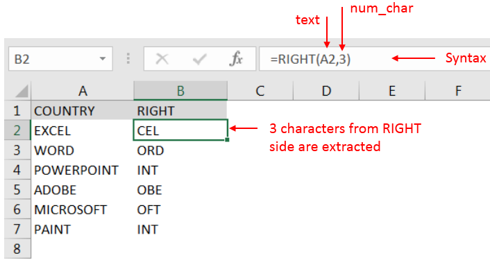
Here, we have a column with Application names and there is requirement of extraction of last Right three character.
We will be following RIGHT function as follows:
“text argument”: “A2” is the cell reference from which characters should be extract
“num_char argument”: “3” is the total number of count of characters required from right side

Explanation: We can see in cell “A2” has string as “EXCEL” and right function extracted total 3 characters from a sting and “CEL” is returned as output in cell “B2”
Hope you learnt this Function!
Don’t forget to leave your valuable comments!
If you are liking our articles and want to learn more similar tricks, please Subscribe us or follow us on Social Media by clicking below buttons.

Microsoft Excel “ISBLANK Function” is a Logical Function and it is used to check if cell in question is “BLANK OR NON-BLANK”. “ISBLANK Function” is used as a test to validate if cell contains any…

Microsoft Excel “NOW” function is used to get the current Date and Time. It is very useful function and can be used in many ways.

LEN function is used for counting number of characters in available string. The output of the function returns the count in new cell.

INT function is used to round down the numeric value to nearest integer. INT Function has one required argument i.e. number.

This tutorial explains how to use the IFERROR function in Excel to catch and handle errors. It shows you how to replace errors with a blank cell, a different value, or a custom message. You’ll also learn how to use IFERROR with functions like VLOOKUP and INDEX MATCH, and how it compares to other error-checking functions like IF ISERROR and IFNA

https://youtu.be/HmJL_y93pAs WEEKNUM function helps to calculate the week number of the given date in a year. It considers 1st January as first week by default and through the output for the given input date. Syntax:…