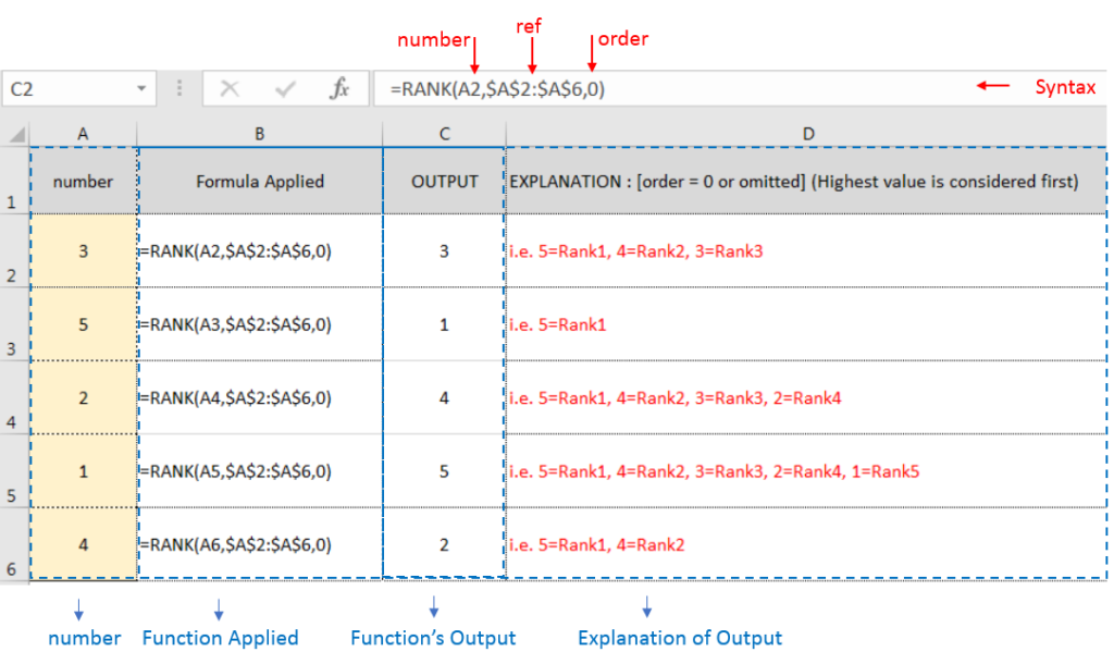
RANK function performs the Ranking in a range or list of numbers. Function returns the rank position and can assigned as Highest or Lowest value as 1st rank as per order argument.
Syntax:
=RANK(number,ref,[order])
number argument is used to give number value for which ranking is required
ref argument is used to give range or list of values from which rank to measure
[order] is optional argument and Value 0 or 1 can be given as per below requirements:
[order] = 0 or omitted: Highest value will be Ranked as 1st position (example: Value 5=Rank1, 4=Rank2, 3=Rank3, 2=Rank4, 1=Rank5 and so on)
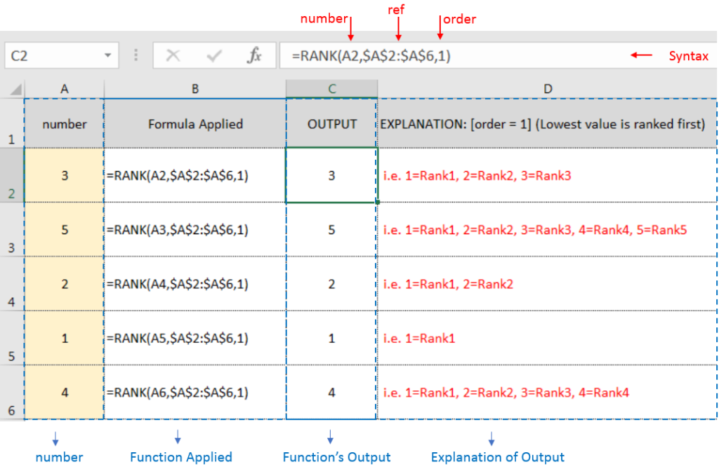
[order] = 1: Lowest value will be Ranked as 1st position (example: Value 1=Rank1, 2=Rank2, 3=Rank3, 4=Rank4, 5=Rank5 and so on)

Example 2: RANK function with [order = 1] (Lowest value is ranked first)

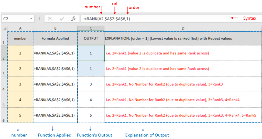
Example 3: RANK function with [order = 1] (Lowest value is ranked first) with Repeat values

If list of values or ref argument has duplicate values, ranking for those values will be same across
Hope you learnt this Function,
Don’t forget to leave your valuable comments!
If you liked this article and want to learn more similar tricks, please Subscribe us or follow us on Social Media by clicking below buttons:

RIGHT function is used for extracting the “Right Most” characters from the available string in Microsoft excel. Function returns value to new string.

Learn an easy way to add pictures directly into a cell using the new IMAGE function! For a long time, adding pictures to Excel was tricky and time-consuming. But now, with the IMAGE function, you…

This step-by-step tutorial empowers you to leverage Power Query’s robust filtering capabilities. Learn to filter by date, text, numbers, and more, streamlining your workflow and unlocking deeper insights from your data. Watch now and elevate your Excel expertise!

ROWS function is used to get the total count of rows in an array or in cells range in an excel worksheet.

SUMIF function is used to get the “total sum” for number of times the criteria across range is met. SUMIF Function has two required arguments.

Microsoft Excel is a useful tool for analyzing data and conducting statistical research. The program includes numerous functions for performing various statistical calculations. One of the essential measures Excel supports is the weighted average.