EXCEL FUNCTION – COUNTIF
Excel Function COUNTIF
COUNTIF Excel Function is also one of the most used function in excel. This helps the user to calculate the number of counts based on single logic given by the user. You can use this function for multiple purposes like:
1. Counting the occurrence in an excel range if meets a criteria i.e. exact value matching, partial value matching, more than or less than of a numeric value
2. Check whether one value exist in other range
3. Count the occurrence if equal to either of values etc.
Excel Function Syntax
Below is the syntax for COUNTIF Function in excel:
1. =COUNTIF(Range,Criteria) Parameters:
– Range: It is an excel range in which you want to count the occurrence of your criteria.
– Criteria: This is a criteria basis on occurrence in the range being counted
When should you use COUNTIF Function
COUNTIF can be used for multiple purposes like
– When you want to count the occurrence of single logic in an excel range
– Also you can use to verify whether one cell value exist in other range. It helps to match one excel range to another range
– You can also count of a value when a criteria in excel range matches, contains, not equal to etc. via wild characters (will discuss this further)
– You can use this function as a logical argument to check if True or False. This can help you in conditional formatting
Things To Remember
– Works with Single Logic and one range (either row or column)
– COUNTIFS can be used for multiple logics
– If your excel range is linked to other workbook, then this function will return #value error when workbook is closed
– Double quotes (” “) should be used when you are using wild characters or not linking the Criteria to Proper Text or Value instead of Excel Cell
Let's Learn COUNTIF with Examples
- Count in a range when exactly values matches with string
Below we are using sales data which contains revenue details for different clients. So here we are going to count the values for particular state.
Suppose you want to count the sales made to clients who belong to state”VA”. So you need to write COUNTIF formula as
=COUNTIF(D:D,"VA")
Here my state details are available in Column D. That’s why I selected D:D range and then typed “VA” as text. So function will check the range and count the occurrence of “VA” state in the given range and retunr the number of count.
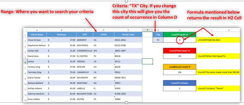
You can link the criteria to Cell as shown in below image and get the results:
- Count in a range when value is not equal to given criteria in an Excel Range
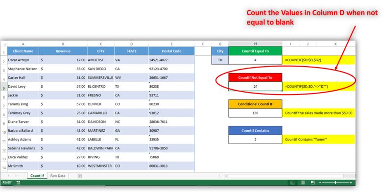
Now suppose you want to count the cells which are not equal to blank cells or any other value in an excel range. You may use this syntax:
=COUNTIF($D:$D,"<>"&"")
Here “<>” is a wild character which is being used for “Not Equal” Criteria and “&” is used to connect one string to another. So here I am using & to connect “<>” with my criteria “” (Non Blank Cells). You can use any string or value or cell to count cells in a range when not equal to. Below are few more criteria examples:
– Count when not equal to
“<>”&””
– Count when not equal to value available in cell G2
“<>”&G2
– Count when not equal to State “VA”
“<>”&”VA”
- Count in a range (here Column B) when value is more than of numeric value
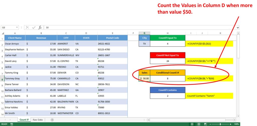
Now suppose you want to count the cells which are more than a numeric value in an excel range. You may use this syntax. Here we are counting the clients who paid more than $50 by checking Column B
=COUNTIF($B:$B,">"&50)
Similar to above example, we are using wild character “>” when more than. You can use different wild characters for counting the numbers in an excel range
– Count when more than 50
“>”&50
– Count when more than to value available in cell G8
“>”&G8
– Count when less than 50
“<”&50
– Count when less than to value available in cell G8
“<”&G8
You can use combination of “>=” or “<=” for when value equals & more than or equals & less than respectively
- Count in a range (here Column A) when value contains particular string
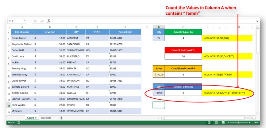
Now suppose you want to count the cells when cell contains particular string in an excel range. You may use this syntax. Here we are counting the clients whose name contains “Tamm” Column A
=COUNTIF($A:$A,"*"&"Tamm"&"*")Similar to above example, we are using wild character “*”&Value/Cell&”*”. This is used to check the range, if contains. Here are few more syntax which are mostly used
– Count when cell value begins with
“Tamm”&”*”
G11&”*”
– Count when cell value ends with
“*”&“Tamm”
“*”&G11
– Count when cell contains
“*”&“Tamm”&”*”
“*”&G11&”*”
Download Practice File
Hope you liked this article. Please comment below for any queries and yes, please do not forget to follow us or subscribe us as below


