How to use “COLUMN” function in Excel

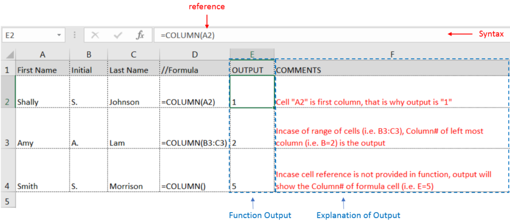
COLUMN function is used to get the column reference number of the excel worksheet.
Function has only one argument i.e. reference, where we need to give cell reference
Syntax Description:
reference argument is used to give the cell reference for which column sequence number is required