Why use dollar sign ($) in Excel formulas – absolute and relative cell references
When creating a formula in Excel, many people get confused by the $ symbol in cell references. But it’s actually very simple. The dollar sign in Excel formula tells Excel whether to keep the reference the same or allow it to change when you copy the formula to other cells. This guide will explain how it works and why it’s helpful.
Understanding Excel cell references is really important. Knowing the difference between absolute, relative, and mixed references will help you get the most out of Excel formulas and functions.
You may have seen the dollar sign ($) in Excel formulas and wondered what it does. You can reference the same cell in four ways: A1, $A$1, $A1, and A$1.
The dollar sign affects how Excel treats the reference when copying or moving the formula. Using $ before a row or column makes an “absolute” reference, which stays the same when copied. Without $, the reference is “relative” and will change.
For a single-cell formula, any reference type works. But if you plan to copy the formula, choosing the right reference type is important. You could guess, but it’s smarter to take a few minutes to learn when to use absolute or relative references in Excel—it’ll make a big difference!
Table of Contents
What is an Excel cell reference?
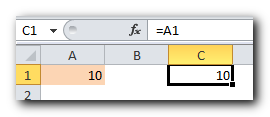
As already mentioned, as long as you write a formula for a single cell, you are free to use any reference type, with or without the dollar sign ($), the result will be the same:

However, if you plan to move or copy the formula across your worksheet, it’s very important to choose the right reference type. This will make sure the formula copies correctly to other cells. The next sections explain each type of cell reference with examples
Note: Besides the A1 reference style (where columns are labeled with letters and rows with numbers), Excel also has the R1C1 style, where both rows and columns are identified by numbers (for example, R1C1 means row 1, column 1).
Since A1 is the default and most commonly used style in Excel, this tutorial will focus only on A1 references. If you’re using the R1C1 style and want to switch, go to File > Options > Formulas and uncheck the R1C1 reference style box.
Excel relative cell reference (without $ sign)
A relative reference in Excel is a cell address without a $ sign, like A1.
When you copy a formula with relative references to another cell, the reference automatically changes based on its new position. By default, all references in Excel are relative. Here’s an example to show how it works.
Say you have this formula in cell B1:
=A1*10
If you copy this formula down to cell B2, it will change to =A2*10 because Excel assumes you want to multiply the value in each row of column A by 10.

If you copy a formula with a relative cell reference to a different column in the same row, Excel will automatically adjust the column reference to match the new position

And if you copy or move an Excel formula with a relative cell reference to another row and another column, both column and row references will change:

As you see, using relative cell references in Excel formulas is a very convenient way to perform the same calculations across the entire worksheet. To better illustrate this, let’s discuss a real-life example.
Using relative reference is Excel - formula example
Let’s say you have a column of prices in USD (in column B), and you want to convert them to EUR. If the USD to EUR rate is 0.93, you can use a simple formula in row 2: =B2*0.93. Notice that this is a relative reference (no $ sign), so it will adjust if copied to other cells.
When you press Enter, Excel will calculate the formula, and the result will show up in the cell right away.
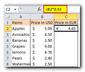
Tip: In Excel, all cell references are relative by default. So, when writing a formula, you can simply click on the cell you want to reference instead of typing it manually.
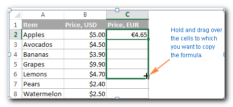
To copy the formula down a column, place your mouse over the fill handle (the small square at the bottom-right corner of the selected cell). When the cursor turns into a thin black cross, click and drag it over the cells you want to fill automatically.
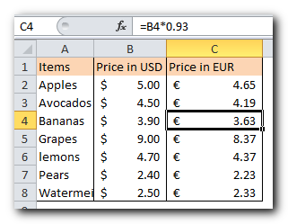
That’s it! The formula is now copied to other cells, with each reference adjusted correctly for each cell. To check that each cell’s value is calculated right, select any cell and look at the formula in the formula bar. In this example, I selected cell C4, and you can see that the cell reference in the formula has adjusted to row 4, just as it should.
Excel absolute cell reference (with $ sign)
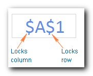
Anabsolute reference in Excel is a cell address with the dollar sign ($) in the row or column coordinates, like $A$1.
The dollar sign fixes the reference to a given cell, so that it remains unchanged no matter where the formula moves. In other words, using $ in cell references allows you to copy the formula in Excel without changing references.
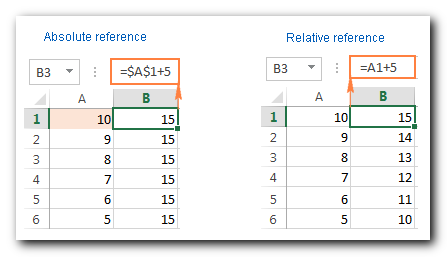
For example, if cell A1 has the number 10 and you use an absolute cell reference ($A$1), the formula =$A$1+5 will always give 15, no matter where you copy the formula.
However, if you use a relative reference (A1) instead, and then copy the formula down the column, each row will calculate a different value. The image below shows this difference
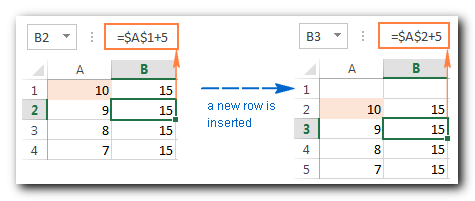
Note. Though we have been saying that an absolute reference in Excel never changes, in fact it does change when you add or remove rows and/or columns in your worksheet, and this changes the location of the referenced cell. In the above example, if we insert a new row at the top of the worksheet, Excel is smart enough to adjust the formula to reflect that change:
In real worksheets, it’s a very rare case when you’d use only absolute references in your Excel formula. However, there are a lot of tasks that require using both absolute and relative references, as demonstrated in the following examples.
In real worksheets, it’s uncommon to use only absolute references in your Excel formulas. Most of the time, you will need to use a mix of both absolute and relative references for different tasks. The following examples will show you how to do this.
Using relative and absolute cell references in one formula
Quite often you may need a formula where some cell references are adjusted for the columns and rows where the formula is copied, while others remain fixed on specific cells. In other words, you have to use relative and absolute cell references in a single formula.
Example 1. Relative and absolute cell references for calculating numbers
In the previous example with USD and EUR prices, you might not want to put the exchange rate directly into the formula. Instead, you can enter the exchange rate in another cell, like C1, and use a dollar sign ($) to make that cell reference absolute in your formula. This way, the reference won’t change when you copy the formula. The following screenshot shows how to do this.
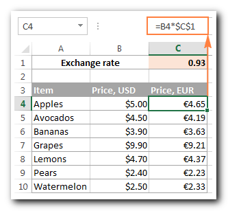
In this formula (B4*$C$1), there are two cell reference types:
- B4 – relativecell reference that is adjusted for each row, and
- $C$1 – absolutecell reference that never changes no matter where the formula is copied.
An advantage of this approach is that your users can calculate EUR prices based on a variable exchange rate without changing the formula. Once the conversion rate changes, all you have to do is to update the value in cell C1.
Example 2. Relative and absolute cell references for calculating dates
Another common use of absolute and relative cell references in one formula is calculating dates in Excel based on today’s date.
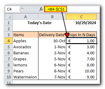
Let’s say you have a list of delivery dates in column B, and you enter today’s date in cell C1 using the TODAY() function. If you want to find out how many days until each item ships, you can use this formula: =B4-$C$1.
Again, we use two types of references in the formula:
- Relative reference for the cell with the delivery date (B4), because you want this reference to change depending on which row the formula is in.
- Absolute reference for the cell with today’s date ($C$1), because you want this reference to stay the same.
In summary, whenever you want to create a static cell reference in Excel that always points to the same cell, remember to add the dollar sign ($) to make it an absolute reference
Excel mixed cell reference
A mixed cell reference in Excel is when either the column letter or the row number is fixed, but not both. For example, $A1 and A$1 are mixed references. Here’s what each one means:
- Absolute column and relative row (like $A1): In this case, the dollar sign ($) in front of the column letter locks the reference to that specific column, so it won’t change when copied to other cells. The row reference, which doesn’t have a dollar sign, will change based on where the formula is copied.
- Relative column and absolute row (like A$1): Here, the row reference is fixed with the dollar sign, so it will stay the same no matter where the formula is copied. The column reference will change based on its new position.
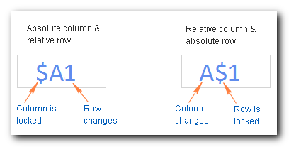
So, mixed references let you control which part of the reference stays the same and which part can change!
Below you will find an example of using both mixed cell reference types that will hopefully make things easier to understand.
Using a mixed reference in Excel - formula example
In this example, we will use our currency conversion table again, but this time we’ll convert dollar prices to several other currencies using just one formula!
First, enter the conversion rates in row 2, as shown in the screenshot below. Then, write a single formula for the top-left cell (C5 in this case) to calculate the EUR price:
=$B5*C$2
Here, $B5 refers to the dollar price in the same row, and C$2 refers to the USD to EUR conversion rate. This way, you can easily convert the prices to different currencies with one formula!
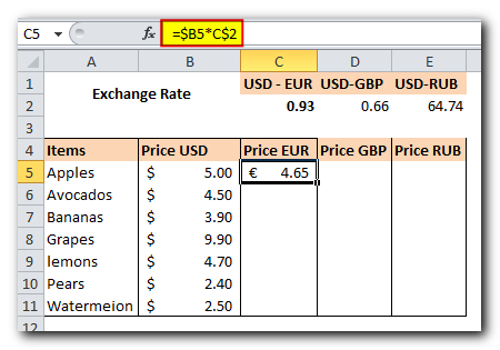
Now, copy the formula down to other cells in column C. Then, you can auto-fill the other columns with the same formula by dragging the fill handle. As a result, you will have three different price columns calculated correctly based on the corresponding exchange rate in row 2.
To check this, select any cell in the table and look at the formula in the formula bar.
For example, if we select cell D7 (in the GBP column), we see the formula =$B7*D$2. This formula takes the USD price from B7 and multiplies it by the value in D2, which is the USD to GBP conversion rate—exactly what you need!
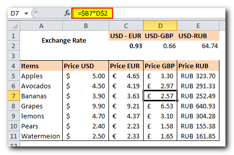
Next, copy the formula down to the other cells in column C. Then, you can auto-fill the other columns with the same formula by dragging the fill handle. This will give you three different price columns, all calculated correctly based on the exchange rates in row 2.
To check your work, select any cell in the table and look at the formula in the formula bar.
For example, if you select cell D7 (in the GBP column), you will see the formula =$B7*D$2. This formula takes the USD price from B7 and multiplies it by the value in D2, which is the USD to GBP conversion rate—just what you need!
How to reference an entire column or row in Excel
When you’re working with an Excel worksheet that has a varying number of rows, you might want to reference all the cells in a specific column. To do this, just type the column letter twice with a colon in between, like this: A:A.
- Whole-Column Reference
Just like cell references, an entire column reference can be either absolute or relative:
– **Absolute column reference**: This is written as `$A:$A`. The dollar sign ($) locks the reference to that specific column, so it won’t change when you copy the formula to other cells.
– **Relative column reference**: This is written as `A:A`. The reference will change if you copy or move the formula to another column, but it will stay the same if you copy the formula to other cells in the same column.
- Whole-Row Reference
To refer to an entire row, you use the same idea but type the row numbers instead of the column letters:
– **Absolute row reference**: This looks like `$1:$1`. The dollar sign locks the reference to that specific row.
– **Relative row reference**: This looks like `1:1`. This reference will change if you copy or move the formula to another row but will stay the same if copied within the same row.
You can also create a mixed reference for an entire column or row, like `$A:A` or `$1:1`, respectively. However, I say “in theory” because I can’t think of any practical use for these mixed references, though Example 4 shows that formulas with them work just fine!
Example 1. Excel entire-column reference (absolute and relative)
Let’s say you have some numbers in column B, and you want to find their total and average. The problem is that new rows are added to the table every week, so using a regular SUM() or AVERAGE() formula for a fixed range of cells isn’t the best approach. Instead, you can reference the entire column B:
- To calculate the total: =SUM($B:$B). Here, the dollar sign ($) makes it an absolute whole-column reference, locking the formula to column B.
- To calculate the total with a relative reference: =SUM(B:B). This formula doesn’t have a dollar sign, so it’s a relative whole-column reference that will change if you copy the formula to other columns.
TIP: When writing the formula, you can click on the column letter to automatically add the entire-column reference. Just like with cell references, Excel will insert a relative reference (without the $ sign) by default.
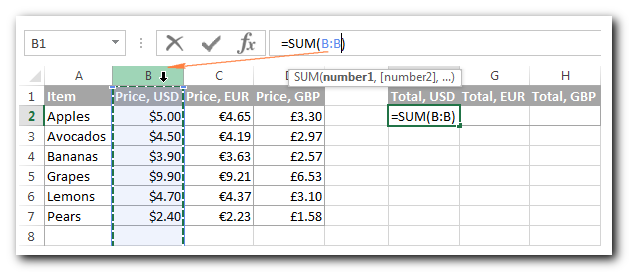
In the same fashion, we write a formula to calculate the average price in the whole column B:
=AVERAGE(B:B)
In this example, we are using a relative entire-column reference, so our formula gets adjusted properly when we copy it to other columns:
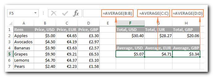
Note. When using an entire-column reference in your Excel formulas, never input the formula anywhere within the same column. For example, it might seem like a good idea to enter the formula =SUM(B:B) in one of the empty bottom-most cells in column B to have the total at the end of the same column. Don’t do this! This would create a so-called circular reference and the formula would return 0.
Example 2. Excel entire-row reference (absolute and relative)
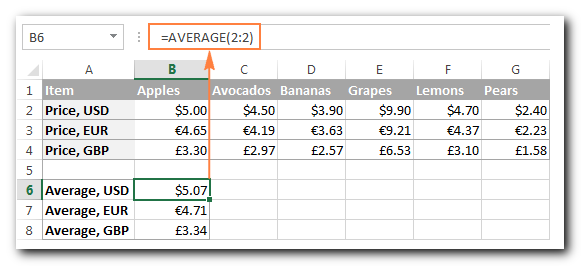
If the data in your Excel sheet is organized in rows rather than columns, then you can reference an entire row in your formula. For example, this is how we can calculate an average price in row 2:
=AVERAGE($2:$2) – an absolute whole-row reference is locked to a specific row by using the dollar sign ($).
=AVERAGE(2:2) – a relative whole-row reference will change when the formula is copied to other rows.
In this example, we need a relative entire-row reference because we have 3 rows of data and we want to calculate an average in each row by copying the same formula:
Example 3. How to refer to an entire column excluding the first few rows
This is a common issue because the first few rows in a worksheet often contain introductory notes or explanations that you don’t want to include in your calculations. Unfortunately, Excel doesn’t allow references like B5:B, which would include all rows in column B starting from row 5. If you try to use that kind of reference, your formula will likely return a #NAME error.
Instead, you can specify a maximum row number so that your reference includes all possible rows in that column. In Excel 2007 and later versions (like Excel 2010, 2013, and 2016), there are 1,048,576 rows and 16,384 columns. In earlier versions of Excel, the maximum was 65,536 rows and 256 columns.
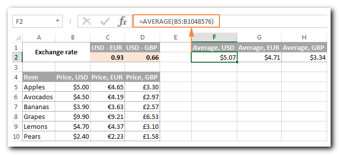
To find the average for each price column in the table below (columns B through D), you would enter the following formula in cell F2 and then copy it to cells G2 and H2
=AVERAGE(B5:B1048576)
Example 4. Using a mixed entire-column reference in Excel
As I mentioned earlier, you can create mixed entire-column or entire-row references in Excel:
- Mixed column reference: like $A:A
- Mixed row reference: like $1:1
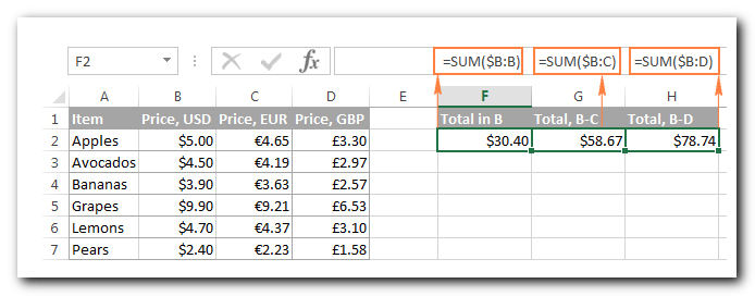
Now, let’s see what happens when you copy a formula with these references to other cells. For example, if you enter the formula =SUM($B:B) in cell F2 and then copy it to the adjacent cell G2, the formula changes to =SUM($B:C). This happens because the first B is fixed with the $ sign, while the second reference (C) is not fixed.
As a result, this formula will add up all the numbers in both columns B and C. While this behavior might not have much practical use, it’s good to know how it works!
How to switch between absolute, relative, and mixed references (F4 key)
When you write an Excel formula, you can manually type the $ sign to change a relative cell reference to absolute or mixed. However, you can also use the F4 key to make this faster. Here’s how to use the F4 shortcut:
- Select the cell with the formula.
- Enter Edit mode by pressing the F2 key or by double-clicking the cell.
- Select the cell reference you want to change.
- Press F4 to switch between the four types of cell references.
If you start with a relative cell reference that has no $ sign, like A1, pressing the F4 key repeatedly will cycle through these options:
- Absolute reference with both dollar signs: $A$1
- Absolute row: A$1
- Absolute column: $A1
- Back to the relative reference: A1
This makes it easy to adjust your references quickly!
Note. If you press F4 without selecting any cell reference, the reference to the left of the mouse pointer will get selected automatically and changed to another reference type.
I hope now you fully understand what relative and absolute cell references are, and an Excel formula with $ signs is no longer a mystery. In the next few articles, we will continue learning various aspects of Excel cell references such as referencing another worksheet, 3d reference, structured reference, circular reference, and so on. In the meantime, I thank you for reading and hope to see you on our blog next week!


