Circular reference in Excel – how to check, find, enable, or remove
This quick guide explains what Excel circular references are and why you should be careful when using them. You’ll also learn how to check for, find, and remove circular references in Excel worksheets. If you need to keep a circular reference, it will show you how to turn on and use circular formulas safely
You tried to enter a formula in your Excel sheet, but it’s not working. Instead, Excel is showing you a message about a circular reference. Is that why you’re here? 🙂
Thousands of people run into this issue every day because they accidentally make an Excel formula try to calculate its own cell. When this happens, Excel gives the following error message:
Be careful! We found one or more circular references in your workbook, which might make your formula calculate incorrectly.”
In simple terms, Excel is saying: “Hey, I might get stuck going in circles. Are you sure you want me to keep going?”
As you can see, circular references in Excel can be tricky, and it’s usually best to avoid them when you can. However, there might be rare situations where a circular reference is the only way to get the job done.
Table of Contents
What is a circular reference in Excel?
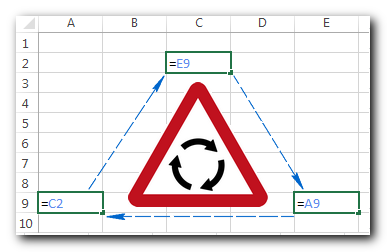
When an Excel formula refers back to its own cell, either directly or indirectly, it creates a circular reference.”
For example, if you click on cell A1 and type =A1, this would create a circular reference. Any other formula that points back to A1, like =A1*5 or =IF(A1=1, “OK”), would also create a circular reference.
As soon as you press Enter to complete a formula like this, you’ll see a warning message pop up.

Why does Microsoft Excel warn you? Because circular references can go in endless loops, causing Excel to slow down as it keeps calculating without stopping.
After you see this warning, you can click “Help” to learn more or close the message by clicking “OK” or the “X” button. When you close the message, Excel will either show a zero (0) or the last value it calculated in the cell. Sometimes, a formula with a circular reference can finish calculating before it starts looping, and in that case, Excel will show the last value it calculated successfully.
Note. In many cases, when you enter more than one formula with a circular reference, Excel doesn’t display the warning message repeatedly.
But why would anyone want to create a formula that only causes problems? Of course, no one would purposely enter a circular formula like that! However, you might accidentally create a circular reference without realizing it. Here’s a common example:
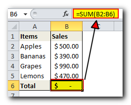
Let’s say you’re trying to add up values in column A using a regular SUM formula. If you accidentally include the total cell itself (like B6 in this example), a circular reference is created.
If circular references are turned off in Excel (which is the default), you’ll see the error message we just talked about. But if iterative calculations are turned on, the circular formula will simply return 0, as shown in the example screenshot.
In some cases, one or more blue arrows can also appear in your spreadsheet all of a sudden, so you might think your Excel has gone mad and is about to crash.
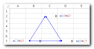
These arrows are just Trace Precedents or Trace Dependents, which show which cells impact or are impacted by the active cell. We’ll go over how to show and hide these arrows soon.
By now, you might think that Excel circular references are completely useless and risky, and wonder why Excel hasn’t removed them entirely. However, in some rare situations, using a circular reference can be helpful because it provides a shorter, cleaner solution—or sometimes it’s the only option. The following example shows one such formula.
Using an Excel circular reference - formula example
In one of our earlier guides, we explained how to add today’s date in Excel. Most of the questions in the comments were about adding a timestamp that doesn’t change every time the sheet is reopened or recalculated. I hesitated to answer because the only way I know to do this uses circular references, which should be handled carefully. But let’s look at a common example…
Imagine you have a list of items in column A and you enter the delivery status in column B. When you type “Yes” in column B, you want the current date and time to show up automatically in column C on the same row as a permanent timestamp.
Using a simple NOW() formula won’t work because this function updates itself each time the sheet recalculates. One possible solution is to use nested IF functions with a circular reference in the second IF.
=IF(B2=”yes”, IF(C2=”” ,NOW(), C2), “”)
Where B2 is the delivery status, and C2 is the cell where you want a timestamp to appear.
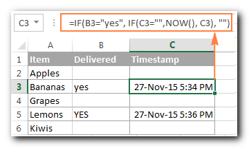
In the formula above, the first IF function checks cell B2 for “Yes” (or any other text you set in the formula). If it finds this text, it runs the second IF; if not, it just returns an empty cell.
The second IF is a circular formula. It grabs the current date and time only if cell C2 is empty, which allows it to keep any existing timestamps unchanged.
Note. For this Excel circular formula to work, you should allow iterative calculations in your worksheet, and this is exactly what we are going to discuss next.
How to enable / disable circular references in Excel
As mentioned before, iterative calculations are usually turned off in Excel by default. Here, “iteration” means Excel repeats calculations until a certain condition is met. For circular formulas to work, you need to turn on iterative calculations.
In Excel 2010 and newer versions, go to File > Options, then select Formulas. Under Calculation options, check the box that says Enable iterative calculation.
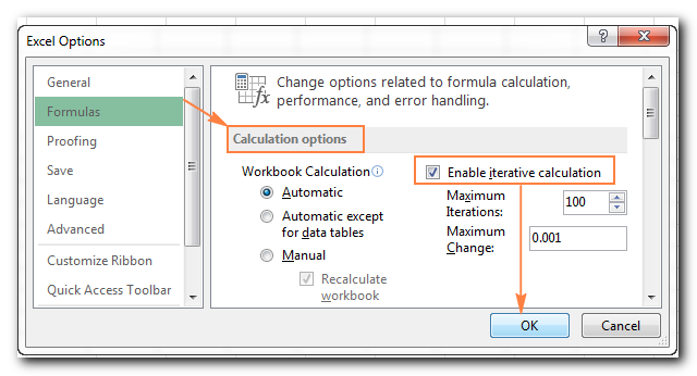
In Excel 2007, go to the Office button > Excel Options > Formulas > Iteration area.
In Excel 2003 and earlier, find the Iterative Calculation option under Menu > Tools > Options > Calculation tab.
When you enable iterative calculations, you need to set two options:
- Maximum Iterations box: This tells Excel how many times the formula should recalculate. The more times it calculates, the longer it takes.
- Maximum Change box: This sets the maximum difference between calculation results. A smaller number gives you a more accurate result, but it takes longer for Excel to finish calculating.
The default settings are 100 for Maximum Iterations and 0.001 for Maximum Change. This means Excel will stop calculating your circular formula after either 100 iterations or when the change is less than 0.001, whichever happens first.
Why you should avoid using circular references in Excel
As you already know, using circular references in Excel can be tricky and is not usually recommended. Besides causing performance problems and showing a warning message every time you open the workbook (unless iterative calculations are enabled), circular references can lead to other issues that may not be obvious right away.
For example, if you select a cell with a circular reference and accidentally enter formula editing mode (by pressing F2 or double-clicking the cell), then press Enter without changing the formula, it will return zero.
Here’s some advice from many experienced Excel users: try to avoid circular references in your sheets whenever you can.
How to find circular references in Excel
To check your Excel workbook for circular references, perform the following steps:
- Go to the Formulas tab, click the arrow next to Error Checking, and point to Circular References The last entered circular reference is displayed there.
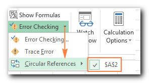
- Click on the cell listed under Circular References, and Excel will bring you exactly to that cell.
As soon as you do this, the status bar will notify you that circular references are found in your workbook and display an address of one of those cells:
If circular references are found in other sheets, the status bar displays only “Circular References” with no cell address.
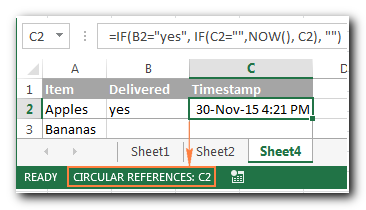
Note. This feature is disabled when the Iterative Calculation option is turned on, so you need to turn it off before you start checking the workbook for circular references.
How to remove circular references in Excel
Unfortunately, Excel doesn’t have a way to remove all circular formulas in a workbook with just one click. To get rid of them, you need to check each circular reference one by one using the steps mentioned earlier. Then, you can either remove the circular formula completely or replace it with one or more simpler formulas.
How to trace relationships between formulas and cells
When a circular reference isn’t easy to spot, the Trace Precedents and Trace Dependents features can help by drawing lines that show which cells influence or are influenced by the selected cell.
To see these trace arrows, go to the Formulas tab, then the Formula Auditing group, and click one of these options:
- Trace Precedents: This shows the cells that provide data to a formula, drawing lines to indicate which cells affect the selected cell.
- Trace Dependents: This shows the cells that rely on the active cell, drawing lines to indicate which cells are affected by it. In other words, it reveals which cells contain formulas that reference the selected cell.
Alternatively, you can use the following shortcuts:
- Trace Precedents: Alt+T U T
- Trace Dependents: Alt+T U D
To hide the arrows, click the Remove Arrows button that resides right underneath Trace Dependents.
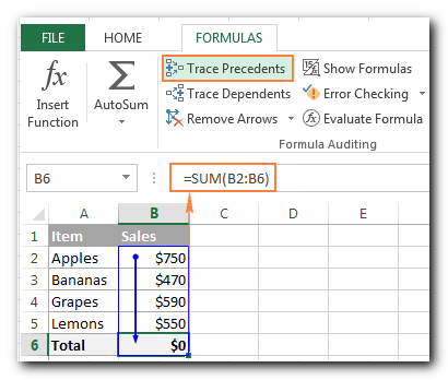
In the example above, the Trace Precedents arrow shows which cells directly provide data to B6. As you can see, cell B6 is included, which creates a circular reference and causes the formula to return zero. This one is easy to fix—just change B6 to B5 in the SUM formula: =SUM(B2).
Other circular references might not be so clear and could require more thought and calculation to resolve.
That’s how you handle circular references in Excel. I hope this short tutorial has helped you understand this tricky topic, and now you can do more research to learn even more. Thank you for reading, and I look forward to seeing you on our blog next week.


