CHOOSEROWS function in Excel to extract rows from array
In this tutorial, we will explore the CHOOSEROWS function in Excel 365 and how to use it in real life.
Imagine you have a big Excel sheet with hundreds of rows, and you need to pick specific ones—like all odd or even rows, the first 5, or the last 10. The thought of copying and pasting or writing VBA code might already feel frustrating. But don’t worry! There’s an easier way. The CHOOSEROWS function can do this for you quickly and easily.
Table of Contents
Excel CHOOSEROWS function
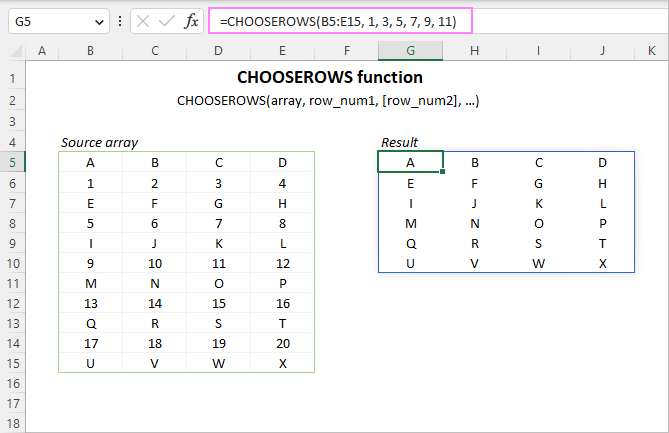
The CHOOSEROWS function in Excel is used to extract the specified rows from an array or range.
The syntax is as follows:
Where:
Array (required) – the source array.
Row_num1 (required) – an integer representing the numeric index of the first row to return.
Row_num2, … (optional) – index numbers of additional rows to return.
Here’s how the CHOOSEROWS function works in Excel 365:
CHOOSEROWS function availability
The CHOOSEROWS function is only available in Excel for Microsoft 365 (Windows and Mac) and Excel for the web.
How to use CHOOSEROWS function in Excel
To extract specific rows from a set of data, create a CHOOSEROWS formula like this:
- Array: This is the data you want to pull rows from. It can be a range of cells or a set of values from another formula.
- Row number (row_num): This tells Excel which row to pick.
- Use a positive number to select a row from the start.
- Use a negative number to select a row from the end.
- You can list multiple row numbers separately or as an array (a group of numbers inside curly brackets {}).
Since CHOOSEROWS is a dynamic array function, it automatically fills the needed space in your sheet. Just type the formula in one cell, and Excel will spread the result across the required rows and columns. This automatic expansion is called a spill range.
For example, to get rows 2, 4, 6, 8 and 10 from the range A4:D13, the formula is:
Alternatively, you can use an array constant such as {2,4,6,8,10} or {2;4;6;8;10} to specify the desired rows:
=CHOOSEROWS(A4:D13, {2,4,6,8,10})
Or
=CHOOSEROWS(A4:D13, {2;4;6;8;10})
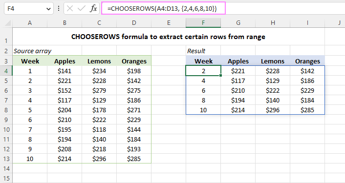
Another way to provide the row numbers is to enter them into separate cells. Then, you can use these cell references in your formula—either listing each one separately or using a range of cells.
For example:
=CHOOSEROWS(A4:D13, F4, G4, H4)
or
=CHOOSEROWS(A4:D13, F4:H4)
The benefit of this method is that you can change the rows you want by simply updating the numbers in those cells, without needing to edit the formula itself.
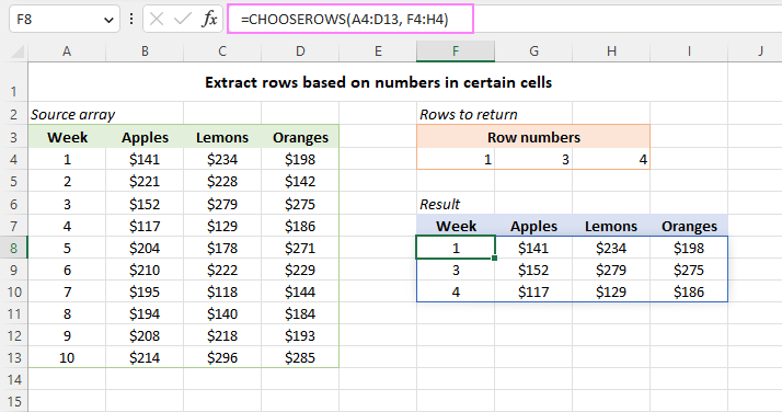
Below we will discuss a few more CHOOSEROWS formula examples to handle more specific use cases.
Return rows from the end of an array
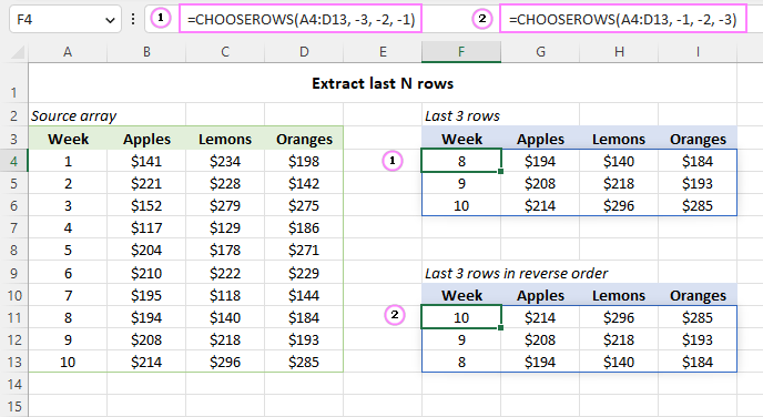
To quickly get the last few rows from a range, use negative numbers for the row numbers. A negative number tells Excel to count from the end of the array.
For example, to get the last 3 rows from the range A4:D13, use:
This returns a 3-row array, with rows in the same order as in the original range.
If you want the last 3 rows in reverse order (from bottom to top), change the order of the numbers:
=CHOOSEROWS(A4:D13, -1, -2, -3)
Extract every other row from an array in Excel
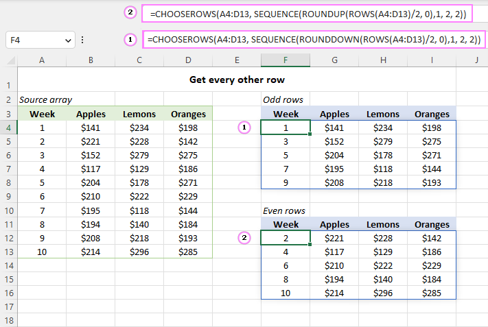
To pick every other row from a range, you can use CHOOSEROWS along with other functions. The formula is slightly different depending on whether you want odd or even rows.
To get odd rows (like 1, 3, 5, …), use this formula:
This selects every first, third, fifth row, and so on.
To get even rows (like 2, 4, 6, …), use this formula:
=CHOOSEROWS(A4:D13, SEQUENCE(ROUNDDOWN(ROWS(A4:D13)/2, 0), 1, 2, 2))
This picks every second, fourth, sixth row, and so on.
These formulas work automatically, so if your data size changes, they will still return the correct rows.
How this formula works:
In simple terms, the CHOOSEROWS function picks rows using a list of numbers created by the SEQUENCE function. Here’s how it works step-by-step:
- Count the rows: First, use the ROWS function to find the total number of rows in your data.
- Divide by 2: Since you want either odd or even rows, divide the total number by 2.
- Round to a whole number: If the division does not result in a whole number (for example, if you have an odd number of rows), use ROUNDUP or ROUNDDOWN to round it to a whole number. This is important because the SEQUENCE function needs an integer.
- Generate the list: The resulting number is then used by the SEQUENCE function to create a list of row numbers that CHOOSEROWS will use.
- Example: If your data range has 10 rows, dividing by 2 gives 5. Since 10 is even, both ROUNDUP(10/2, 0) and ROUNDDOWN(10/2, 0) return 5.
In short, CHOOSEROWS returns the rows specified by the sequence of numbers, making it easy to extract odd or even rows from your data.
The number we calculated earlier is used in the SEQUENCE function to create a list of row numbers.
For odd rows:
SEQUENCE(5, 1, 1, 2)
This creates a list starting at 1 and increasing by 2 each time:
{1;3;5;7;9}
For even rows:
SEQUENCE(5, 1, 2, 2)
This starts at 2 and also increases by 2:
{2;4;6;8;10}
This list of numbers is then passed to the CHOOSEROWS function, which picks those rows from the given range.
For example, to select odd rows:
=CHOOSEROWS(A4:D13, {1;3;5;7;9})
This extracts rows 1, 3, 5, 7, and 9 from A4:D13 automatically!
Reverse the order of rows in an array
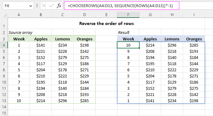
To flip an array vertically (reverse the order of the rows), you can combine the CHOOSEROWS and SEQUENCE functions. For example:
Here’s how it works:
- Count the rows:
The formula ROWS(A4:D13) counts how many rows are in the range. - Create a sequence:
The SEQUENCE function creates a list of numbers from 1 to that count. The other SEQUENCE settings (columns, start, step) default to 1. - Multiply by -1:
By multiplying the sequence by -1, you get negative numbers (like -1, -2, -3, …). Negative numbers tell CHOOSEROWS to count from the bottom up. - Flip the order:
CHOOSEROWS uses these negative numbers to reverse the order of the rows, so the first row becomes the last and the last becomes the first.
This simple trick flips the order of items in each column from top-to-bottom.
Extract rows from multiple arrays
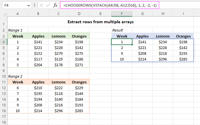
To get specific rows from two or more non-contiguous ranges, you first combine them using the VSTACK function, and then pass the merged range to CHOOSEROWS.
For example, to extract the first two rows from the range A4:D8 and the last two rows from the range A12:D16, use this formula:
Get rows based on a string containing row numbers
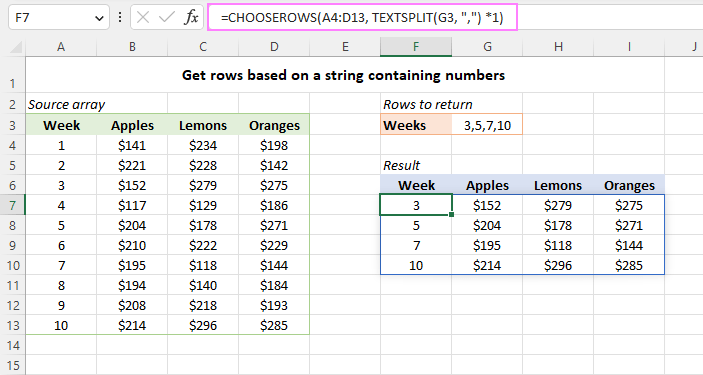
This example shows you how to pick certain rows by getting the row numbers from a text string.
Imagine you have a cell (G3) with comma-separated numbers that list the rows you want, for example: 3,5,7,10.
- Split the text:
Use the TEXTSPLIT function to break the text into separate pieces using the comma as the divider: - =TEXTSPLIT(G3, “,”)
This creates an array of text values like: {“3”, “5”, “7”, “10”}.
- Convert text to numbers:
To turn these text values into numbers, multiply by 1 (or add 0): - =TEXTSPLIT(G3, “,”) * 1
Now you have a numeric array: {3,5,7,10}.
- Use with CHOOSEROWS:
Insert the formula into the CHOOSEROWS function as the row numbers argument: - =CHOOSEROWS(A4:D13, TEXTSPLIT(G3, “,”) * 1)
This tells Excel to return the rows specified by the numbers in G3 as a single array.
In short, you extract the row numbers from a text string and then use them to pull out the desired rows from your data.
That’s how to use the CHOOSEROWS function in Excel to return particular rows from a range or array. Thank you for reading and I hope to see you on our blog next week!


