Excel CHOOSE function
The tutorial explains how to use the CHOOSE function in Excel, showing you the basics and some interesting examples. While CHOOSE might seem simple on its own, when you combine it with other functions, it can be powerful. Essentially, the CHOOSE function helps you pick a value from a list based on its position. The tutorial also covers some advanced ways to use CHOOSE that you might find very useful.
Table of Contents
Excel CHOOSE function - syntax and basic uses
The CHOOSE function in Excel lets you pick a value from a list based on its position.
You can use this function in Excel 365, 2019, 2016, 2013, 2010, and 2007.
The format of the CHOOSE function is as follows:
CHOOSE (index_num, value1, [value2], …)
Where:
Index_num (required) – the position of the value to return. It can be any number between 1 and 254, a cell reference, or another formula.
Value1, value2, … – a list of up to 254 values from which to choose. Value1 is required, other values are optional. These can be numbers, text values, cell references, formulas, or defined names.
Here’s an example of a CHOOSE formula in the simplest form:
=CHOOSE(3, “Andrew”, “Emma”, “Herry”, “Neal”)
The formula returns “Herry” because index_num is 3 and “Herry” is the 3rd value in the list:

Excel CHOOSE function - 3 things to remember!
The CHOOSE function is straightforward and easy to use, so you shouldn’t have much trouble adding it to your worksheets. However, if the result you get isn’t what you expected, it might be due to a few reasons:
- You can only choose from up to 254 values.
- If the position number (index_num) is less than 1 or more than the number of values in the list, you’ll get a #VALUE! error.
- If the position number is a fraction, it will be rounded down to the nearest whole number.
How to use CHOOSE function in Excel - formula examples
The examples below show how CHOOSE can work with other Excel functions to do more powerful tasks and offer alternative solutions to common problems, even those that many people think are impossible to solve.
Excel CHOOSE instead of nested Ifs
One of the common tasks in Excel is to return different values based on a specific condition. Usually, people use a nested IF statement for this, but the CHOOSE function can be a faster and simpler alternative.
Example 1. Return different values based on condition
Supposing you have a column of student scores and you want to label the scores based on the following conditions:
Result | Score |
Poor | 0 – 50 |
Satisfactory | 51 – 100 |
Good | 101 – 150 |
Excellent | over 151 |
=IF(B2>=151, “Excellent”, IF(B2>=101, “Good”, IF(B2>=51, “Satisfactory”, “Poor”)))
Another way is to choose a label corresponding to the condition:
=CHOOSE((B2>0) + (B2>=51) + (B2>=101) + (B2>=151), “Poor”, “Satisfactory”, “Good”, “Excellent”)

How this formula works:
In the index_num argument, you evaluate each condition and return TRUE if the condition is met, FALSE otherwise. For example, the value in cell B2 meets the first three conditions, so we get this intermediate result:
=CHOOSE(TRUE + TRUE + TRUE + FALSE, “Poor”, “Satisfactory”, “Good”, “Excellent”)
Given that in most Excel formulas TRUE equates to 1 and FALSE to 0, our formula undergoes this transformation:
=CHOOSE(1 + 1 + 1 + 0, “Poor”, “Satisfactory”, “Good”, “Excellent”)
After the addition operation is performed, we have:
=CHOOSE(3, “Poor”, “Satisfactory”, “Good”, “Excellent”)
As the result, the 3rd value in the list is returned, which is “Good”.
Example 2. Perform different calculations based on condition
Similarly, you can use the Excel CHOOSE function to perform one calculation out of several possible options, without needing to stack multiple IF statements.
For example, let’s calculate each seller’s commission based on their sales:
Commission | Sales |
5% | $0 to $50 |
7% | $51 to $100 |
10% | over $101 |
With the sales amount in B2, the formula takes the following shape:
=CHOOSE((B2>0) + (B2>=51) + (B2>=101), B2*5%, B2*7%, B2*10%)

Instead of hardcoding the percentages in the formula, you can refer to the corresponding cell in your reference table, if there is any. Just remember to fix the references using the $ sign.
=CHOOSE((B2>0) + (B2>=51) + (B2>=101), B2*$E$2, B2*$E$3, B2*$E$4)
Excel CHOOSE formula to generate random data
As you may know, Microsoft Excel has a function called RANDBETWEEN that generates random numbers between the two numbers you choose. By placing RANDBETWEEN inside the index_num argument of CHOOSE, you can create a formula that generates almost any random data you need.
For example, this formula can produce a list of random exam results:
=CHOOSE(RANDBETWEEN(1,4), “Poor”, “Satisfactory”, “Good”, “Excellent”)

The formula is simple: RANDBETWEEN picks a random number from 1 to 4, and CHOOSE returns the matching value from a list of four preset options
Note:- RANDBETWEEN is a volatile function, meaning it recalculates every time you make a change to the worksheet. This causes your list of random values to keep changing. To stop this, you can use the Paste Special feature to replace the formulas with their actual values
CHOOSE formula to do a left Vlookup
If you’ve ever used VLOOKUP in Excel, you know it can only search in the left-most column. But if you need to return a value from a column to the left of the one, you’re looking up, you can either use the INDEX/MATCH combination or trick VLOOKUP by nesting the CHOOSE function inside it. Here’s how:
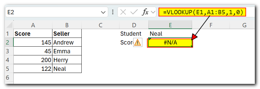
Let’s say you have a list of scores in column A and student names in column B, and you want to find a student’s score. Since the scores are in a column to the left of the names, a regular VLOOKUP formula would give you a #N/A error.

To fix this, get the CHOOSE function to swap the positions of columns, telling Excel that column 1 is B and column 2 is A:
=CHOOSE({1,2}, B2:B5, A2:A5)
Because we supply an array of {1,2} in the index_num argument, the CHOOSE function accepts ranges in the value arguments (normally, it doesn’t).
Now, embed the above formula into the table_array argument of VLOOKUP:
=VLOOKUP(E1,CHOOSE({1,2}, B2:B5, A2:A5),2,FALSE)

CHOOSE formula to return next working day
If you’re unsure whether you need to go to work tomorrow or can enjoy your weekend at home, the Excel CHOOSE function can help you figure out when your next workday is.
If your workdays are Monday to Friday, the formula looks like this
=TODAY()+CHOOSE(WEEKDAY(TODAY()),1,1,1,1,1,3,2)

While it might seem tricky at first, the formula’s logic is actually easy to understand:
WEEKDAY(TODAY()) gives a number for today’s day of the week, from 1 (Sunday) to 7 (Saturday). This number is used in the CHOOSE formula’s index_num argument.
The values (1,1,1,1,1,3,2) tell the formula how many days to add to today’s date. If today is Sunday to Thursday (1 to 5), you add 1 day to get the next day. If today is Friday (6), you add 3 days to jump to Monday. If today is Saturday (7), you add 2 days to also reach Monday. Yep, it’s that simple!
CHOOSE formula to return a custom day/month name from date
If you want to get a day name in the standard format, like the full name (Monday, Tuesday, etc.) or short name (Mon, Tue, etc.), you can use the TEXT function, as shown in the example: Get day of week from date in Excel.
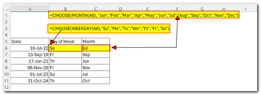
But if you want to return a day of the week or a month name in a custom format, you can use the CHOOSE function like this:
To get a day of the week:
=CHOOSE(WEEKDAY(A2),”Su”,”Mo”,”Tu”,”We”,”Th”,”Fr”,”Sa”)
To get a month:
=CHOOSE(MONTH(A2), “Jan”,”Feb”,”Mar”,”Apr”,”May”,”Jun”,”Jul”,”Aug”,”Sep”,”Oct”,”Nov”,”Dec”)
Where A2 is the cell containing the original date.

I hope this tutorial has given you some ideas on how to use the CHOOSE function in Excel to improve your data models. Thank you for reading


