How to Use Array Function in Excel
In this tutorial, you’ll learn how to use Array function in excel, how to enter it properly, and how to use array constants and array functions. Array formulas are a very powerful tool in Excel, allowing you to do multiple calculations with a single formula. One array formula can replace many regular formulas. However, most users—around 90%—have never used them because they seem intimidating to learn. Array formulas are known to be one of the trickiest Excel features to understand. The goal of this tutorial is to make learning them as easy and simple as possible.
Table of Contents
What is an array function in Excel?
Before we dive into array functions and formulas, let’s first understand what the term “array” means. An array is simply a collection of items. These items can be text or numbers, and they can be arranged in a single row, a single column, or across multiple rows and columns.
For example, if you were to organize your weekly grocery list as an Excel array, it might look like this:
{“Milk”, “Eggs”, “Butter”, “Corn flakes”}
Now, if you select cells A1 to D1, type this array in the formula bar with an equal sign (=) at the beginning, and press CTRL + SHIFT + ENTER, Excel will display the items in those cells.

What you have just done is create a one-dimensional horizontal array. Nothing dreadful so far, right?
What is an array Function Excel?
The key difference between an array formula and a regular formula is that an array formula works with multiple values at once, not just one. In other words, an array formula evaluates all the individual values in an array and performs calculations on one or more items based on the formula’s conditions.
Not only can an array formula handle several values at the same time, but it can also return multiple results. So, the output of an array formula is also an array.
Array formulas are available in all versions of Excel, including Excel 2019, 2016, 2013, 2010, 2007, and earlier.
Now, it’s a great time to try creating your first array formula!
Simple example of Excel array Function
Suppose you have some items in column B, their prices in column C, and you want to calculate the grand total of all sales.
Of course, nothing prevents you from calculating subtotals in each row first with something as simple as =B2*C2 and then sum those values:
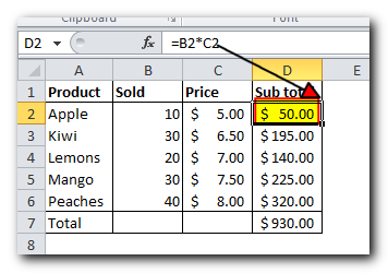
An array formula can save you extra steps by letting Excel store intermediate results in memory, instead of using an extra column. With just one array formula and two quick steps, you can do the same work:
- Select an empty cell and enter this formula: =SUM(B2:B6*C2:C6)
- Press CTRL + SHIFT + ENTER to complete the array formula.
After doing this, Excel will surround the formula with curly braces {}, showing it’s an array formula.
This formula multiplies the values in each row from the ranges B2 to B6 and C2 to C6, then adds up the results to give you a grand total.
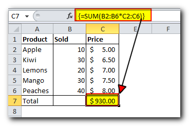
This simple example shows just how powerful an array formula can be. When you’re working with hundreds or even thousands of rows of data, imagine how much time you can save by using a single array formula in one cell instead of creating multiple formulas.
Why use array Function in Excel?
Excel array formulas are a very useful tool for handling complex calculations and tasks. One array formula can replace hundreds of regular formulas. They are especially helpful for tasks like:
- Summing numbers that meet specific conditions, such as adding the N largest or smallest values in a range.
- Summing every other row, or every Nth row or column, as shown in this example.
Counting the number of all characters or specific characters in a range. For example, an array formula can count all characters or any specific ones you choose
How to enter array formula in Excel (Ctrl + Shift + Enter)
As you know, pressing the three keys CTRL + SHIFT + ENTER is the “magic touch” that turns a regular formula into an array formula.
When working with array formulas in Excel, remember these 4 key points:
- After typing the formula and pressing CTRL + SHIFT + ENTER, Excel automatically surrounds the formula with {curly braces}. When you select the cell, you’ll see these braces in the formula bar, indicating that it’s an array formula.
- Manually typing the curly braces around a formula won’t work. You must press CTRL + SHIFT + ENTER to create an array formula.
- Every time you edit an array formula, the curly braces disappear, so you’ll need to press CTRL + SHIFT + ENTER again to save the changes.
- If you forget to press CTRL + SHIFT + ENTER, your formula will act like a regular formula and only process the first value(s) in the array.
Because you need to use CTRL + SHIFT + ENTER for all array formulas, they’re sometimes called CSE formulas.
Use the F9 key to evaluate portions of an array formula
When using array formulas in Excel, you can see how they calculate and store their values (called internal arrays) before showing the final result in a cell. To do this, select part of the formula inside the parentheses, then press the F9 key. This will show the intermediate results. To exit this mode, press the Esc key.
For example, if you want to see the sub-totals of all products in the earlier formula, you would select B2:B6*C2:C6, press F9, and Excel will show you the result of the multiplication for each row
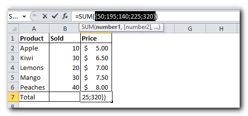
Note. Please pay attention that you must select some part of the formula prior to pressing F9, otherwise the F9 key will simply replace your formula with the calculated value(s).
Single-cell and multi-cell array formulas in Excel
An Excel array formula can return results in either a single cell or multiple cells. If the array formula is entered across a range of cells, it’s called a multi-cell formula. If the array formula is in just one cell, it’s called a single-cell formula.
Some Excel functions are designed to return results across multiple cells, like TRANSPOSE, TREND, FREQUENCY, and LINEST.
Other functions, such as SUM, AVERAGE, AGGREGATE, MAX, and MIN, can calculate array values in a single cell when entered with Ctrl + Shift + Enter.
Here are some examples to show how to use both single-cell and multi-cell array formulas.
Example 1. A single-cell array formula
Let’s say you have two columns showing the number of items sold in two different months, columns B and C, and you want to find the biggest sales increase.
Normally, you would create an extra column (like column D) to calculate the sales change for each product using a formula like =C2-B2, and then use =MAX(D:D) to find the maximum value in that new column.
With an array formula, you don’t need an extra column because it stores the intermediate results in memory. Instead, just enter this formula and press Ctrl + Shift + Enter:
=MAX(C2:C6-B2:B6)
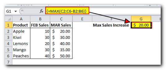
Example 2. A multi-cell array formula in Excel
In the previous SUM example, let’s say you need to calculate a 10% tax for each sale, and you want to do this with just one formula.
First, select the empty cells where you want the results to go, like D2 to D6, and then type this formula into the formula bar:
=B2:B6 * C2:C6 * 0.1
After pressing Ctrl + Shift + Enter, Excel will automatically fill each cell in the selected range with the tax amounts, and you’ll see the results appear in those cells
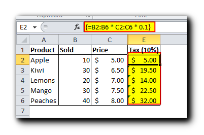
Excel array constants
In Microsoft Excel, an array constant is just a set of fixed values that don’t change when you copy the formula to other cells.
You’ve already seen an example of an array constant with a grocery list earlier in this tutorial. Now, let’s explore the different types of array constants and how to create them.
There are 3 types of array constants:
- Horizontal array constant
A horizontal array constant is a set of values that are arranged in a row. To create one, type the values separated by commas and put them inside curly braces, like this: {1,2,3,4}.
Note: When creating an array constant, you must manually type the opening and closing curly braces.
To enter a horizontal array in your spreadsheet, follow these steps:
- Select the same number of blank cells in a row as the number of values in your array.
- Type the formula ={1,2,3,4} in the formula bar.
- Press Ctrl + Shift + Enter.
You’ll see the values appear across the selected row, similar to this setup
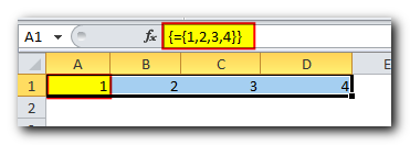
As you see in the screenshot, Excel wraps an array constant in another set of braces, exactly like it does when you are entering an array formula.
- Vertical array constant
A vertical array constant resides in a column. You create it in the same way as a horizontal array with the only difference that you delimit the items with semicolons, for example:
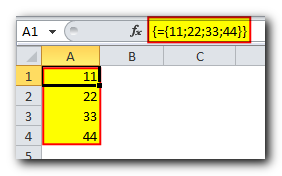
- Two-dimensional array constant
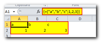
To create a two-dimensional array, you separate each row by a semicolon and each column of data by a comma.
={“a”, “b”, “c”; 1, 2, 3}
Working with Excel array constants
Array constants are a key part of Excel array formulas. Here are some useful tips to help you use them more effectively
Elements of an array constant
An array constant can include numbers, text, Booleans (TRUE or FALSE), and error values, separated by commas or semicolons.
- Numbers can be entered as whole numbers, decimals, or in scientific notation.
- Text values should be surrounded by double quotes (e.g., “Text”).
However, an array constant cannot include other arrays, cell references, ranges, dates, defined names, formulas, or functions.
Naming array constants
To make an array constant easier to use, you can give it a name:
- Go to the Formulas tab, find the Defined Names group, and click Define Name. Or, you can press Ctrl + F3 and then click New.
- In the Name box, type the name you want to give the array.
- In the Refers to box, enter your array constant, with the values inside braces {} and starting with an equal sign =. For example:
={“Su”, “Mo”, “Tu”, “We”, “Th”, “Fr”, “Sa”}
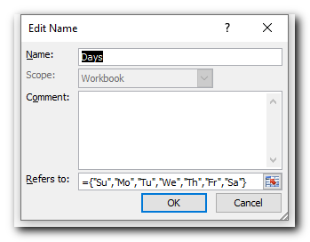
Click OK to save your named array and close the window.
To enter the named array constant in a sheet, select as many cells in a row or column as there are items in your array, type the array’s name in the formula bar preceded with the = sign and press Ctrl + Shift + Enter.
The result should resemble this:

Preventing errors
If your array constant isn’t working properly, check for these common issues:
- Use the correct separator: commas for horizontal arrays and semicolons for vertical arrays.
- Make sure you’ve selected the exact number of cells to match the number of items in your array. If you select too many cells, the extra ones will show #N/A errors. If you select too few, only part of the array will be inserted.
Using array constants in Excel formulas
Now that you are familiar with the concept of array constants, let’s see how you can use arrays in formulas to solve your practical tasks.
Example 1. Sum N largest / smallest numbers in a range
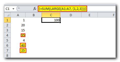
Start by creating a vertical array constant with the numbers you want to sum. For example, to add the 3 smallest or largest numbers in a range, use the array constant {1,2,3}.
Next, use the LARGE or SMALL function:
- In the first parameter, specify the range of cells.
- In the second parameter, include the array constant.
Finally, wrap it in the SUM function like this:
- To sum the largest 3 numbers: =SUM(LARGE(range, {1,2,3}))
- To sum the smallest 3 numbers: =SUM(SMALL(range, {1,2,3}))
Since this is an array formula, remember to press Ctrl + Shift + Enter to get the result.
In a similar fashion, you can calculate the average of N smallest or largest values in a range:
Average of the top 3 numbers: =AVERAGE(LARGE(range, {1,2,3}))
Average of the bottom 3 numbers: =AVERAGE(SMALL(range, {1,2,3}))
Example 2. Array formula to count cells with multiple conditions
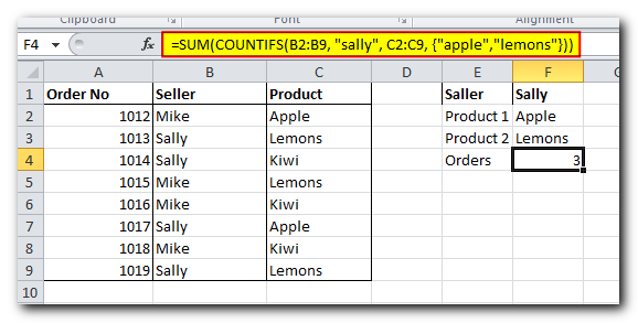
Let’s say you have a list of orders and want to find out how many times a specific seller has sold certain products.
The easiest way to do this is by using a COUNTIFS formula with multiple conditions. However, if you have many products, the COUNTIFS formula can get very long. To keep it simpler, you can combine COUNTIFS with SUM and use an array constant in one or more of the arguments.
For example:
=SUM(COUNTIFS(range1, “criteria1”, range2, {“criteria1”, “criteria2”}))
A real example might be:
=SUM(COUNTIFS(B2:B9, “sally”, C2:C9, {“apples”, “lemons”}))
This formula counts how many times Sally sold either apples or lemons
Our example array only has two elements because we want to show you the method in a simple way. In your actual array formulas, you can include as many elements as you need, as long as the formula doesn’t exceed 8,192 characters in Excel 2019 – 2007 (or 1,024 characters in Excel 2003 and earlier). Keep in mind that large arrays might need a more powerful computer to process them.
Here’s a more advanced array formula example: you can use SUM and VLOOKUP with an array constant to find the sum of all matching values in a table
Double unary operator in Excel array formulas
If you’ve worked with array formulas in Excel, you might have seen a double dash (–) and wondered what it’s for.
The double dash, or double unary operator, is used to turn non-numeric Boolean values (TRUE/FALSE) into numbers (1 and 0) so that Excel’s array functions can work with them.
Here’s an example to explain this better: Let’s say you have a list of dates in column A, and you want to count how many of those dates are in January, no matter the year.
The formula is:
=SUM(–(MONTH(A2:A10)=1))
This is an array formula, so remember to press Ctrl + Shift + Enter.
If you want to check a different month, just change the number. For example, use 2 for February, 3 for March, and so on. You can also make the formula more flexible by entering the month number in a separate cell and referencing it in the formula.
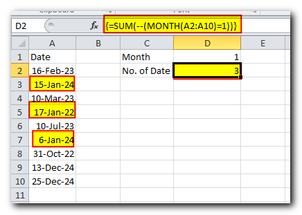
Now, let’s break down how this array formula works in simple steps:
- MONTH function: This function takes the dates in cells A2 through A10 and returns the month for each, producing an array like {2;1;4;2;12;1;2;12;1}. These are the months corresponding to the dates.
- Comparison: Next, each month from the array is compared to the value in cell D1, which is 1 (for January) in this example. This comparison returns an array of TRUE and FALSE values depending on whether the month matches January. So you might get something like {FALSE;TRUE;FALSE;FALSE;FALSE;TRUE;FALSE;FALSE;TRUE}.
- Viewing part of the formula: You can check parts of an array formula by selecting it and pressing F9. This shows what the selected portion calculates.
- Converting to numbers: Excel can’t add TRUE or FALSE, so the double negative (–) is used to convert TRUE into 1 and FALSE into 0. The first negative turns TRUE/FALSE into -1/0, and the second negative flips them to positive 1 and 0. Now, the SUM function can add them up correctly.
If you remove the double negatives, the formula won’t work properly, as Excel wouldn’t understand the TRUE/FALSE values.
I hope this short guide helps you on your journey to mastering Excel array formulas. Next week, we’ll dive into more advanced examples. Stay tuned, and thanks for reading!


