Advance Filter in Excel – how to create and use
This guide explains the basics of advance filter in excel and shows you how to use it to find records that match one or more complicated conditions.
If you’ve read our previous guide, you know that Excel’s regular filter offers different options for filtering text, numbers, and dates. These options work well for many situations, but not all. When the regular filter isn’t enough, you can use the Advanced Filter to set up custom criteria that fit your exact needs.
Excel’s Advanced Filter is especially useful for finding data based on two or more complex conditions. For example, you can use it to find matches and differences between two columns, filter rows that match another list, or find exact matches with the same uppercase and lowercase letters.
Advanced Filter is available in all Excel versions from 365 to 2003. Click the links below to learn more.
Table of Contents
Excel Advanced Filter vs. AutoFilters
Compared to the basic AutoFilter tool, the Advanced Filter works differently in a few important ways.
The AutoFilter in Excel is very simple to use. You just click one button, and it’s ready. Press the Filter button on the ribbon, and you can start filtering your data right away.
The Advanced Filter is not automatic because it doesn’t have a built-in setup. You have to manually set up the list range and criteria range yourself.
With AutoFilter, you can filter data using only 2 conditions, and you enter those conditions directly in the Custom AutoFilter box.
With the Advanced Filter, you can filter rows based on multiple conditions across different columns. You set up these advanced conditions in a separate area of your worksheet.
Below, you’ll find detailed instructions on how to use the Advanced Filter in Excel, plus some examples for filtering text and numbers.
How to create an advance filter in excel
Using Excel’s Advanced Filter is a bit harder than the AutoFilter (as is the case with many ‘advanced’ features 🙂 but it’s definitely worth it. To set up an advanced filter for your sheet, follow these steps.
1. Organize the source data
For the best results, organize your data using these 2 simple rules:
- Add a header row with a unique heading for each column—duplicate headings can confuse the Advanced Filter.
- Make sure there are no blank rows in your data.
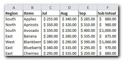
For example, here’s how our sample table looks:
2. Set up the criteria range
Enter your conditions, also called criteria, in a separate area on the worksheet. In theory, the criteria can go anywhere on the sheet, but it’s usually easier to place them at the top and leave one or more blank rows between the criteria and your data.
Advanced criteria notes:
The criteria range must have the same column headings as the table or range you want to filter.
- Criteria on the same row use AND logic (both conditions must be true).
- Criteria on different rows use OR logic (either condition can be true).
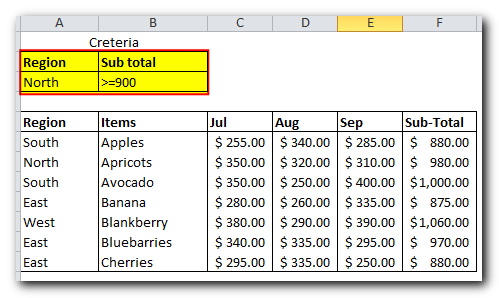
For example, to filter records for the North region with a Sub-total of 900 or more, your criteria range should look like this:
- Region: North
- Sub-total: >=900″
3. Apply Excel Advanced Filter
Once your criteria range is set up, follow these steps to apply an advanced filter:
- Select any cell in your data.
- In Excel 2016, 2013, 2010, or 2007, go to the Data tab, find the Sort & Filter group, and click Advanced.
- In Excel 2003, click the Data menu, then point to Filter, and select Advanced Filter…
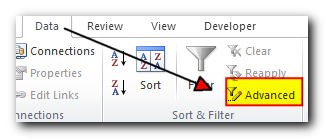
The Excel Advanced Filter dialog box will appear and you set it up as explained below.
4. Configure the Advanced Filter parameters
In the Excel Advanced Filter dialog window, specify the following parameters:
- Action Choose whether to filter the list in place or copy the results to another location.
Selecting “Filter the list in place” will hide the rows that don’t match your criteria.
If you choose “Copy the results to another location”, select the upper-left cell of the range where you want to paste the filtered rows. Make sure the destination range has no data anywhere in the columns because all cells below the copied range will be cleared.
- List range. This is the range of cells you want to filter, and it should include the column headings.
If you selected any cell in your data before clicking the Advanced button, Excel will automatically select the whole data range. If Excel selects the wrong range, click the small Collapse Dialog button next to the List Range box, and then use your mouse to pick the correct range.
- Criteria range. This is the range of cells where you enter your criteria.
Also, there’s a checkbox in the lower-left corner of the Advanced Filter dialog box that lets you show only unique records. This option helps you find all the different items in a column.
In this example, we are filtering the list in place, so set up the Excel Advanced Filter parameters like this:
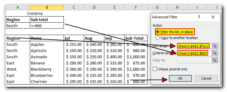
Finally, click OK, and you will get the following result:
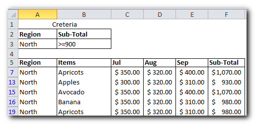
This is great, but you can actually get the same result using the regular Excel AutoFilter, right? However, please don’t leave this page just yet! We’ve only covered the basics of how the Excel Advanced Filter works. Later in the article, you’ll find some examples that can only be done with the Advanced Filter. To help you understand better, let’s learn more about the Advanced Filter criteria first.
Excel Advanced Filter criteria range
As you have just seen, there is no rocket science in using Advanced Filter in Excel. But once you learn the nitty-gritty details of the Advanced Filter criteria, your options will be almost unlimited!
Comparison operators for numbers and dates
In the Advanced Filter criteria, you can compare different numeric values using the following comparison operators.
Comparison operator | Meaning | Example |
= | Equal to | A1=B1 |
> | Greater than | A1>B1 |
< | Less than | A1<B1 |
>= | Greater than or equal to | A1>=B1 |
<= | Less than or equal to | A1<=B1 |
<> | Not equal to | A1<>B1 |
Using comparison operators with numbers is straightforward. In the example above, we used the numeric criteria >=900 to filter records with a Subtotal of 900 or more.
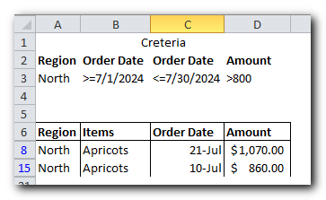
Here’s another example: If you want to show records for the North region for July with an Amount greater than 800, you would set up the following conditions in the criteria range:
- Region: North
- Order date: >=7/1/2016
- Order date: <=7/30/2016
- Amount: >800
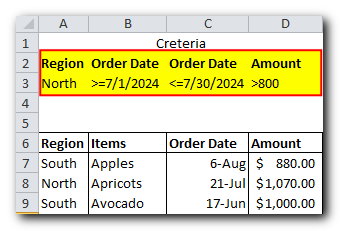
And now, run the Excel Advanced Filter tool, specify the List range (A4:D50) and Criteria range (A2:D2) and you will get the following result:
Advanced filter for text values
Apart from numbers and dates, you can also use the logical operators to compare text values. The rules are defined in the table below.
Criteria | Description |
=”=text” | Filter cells whose values are exactly equal to “text”. |
text | Filter cells whose contents begin with “text”. |
<>text | Filter cells whose values are not exactly equal to “text” (cells containing “text” as part of their contents will be included in the filter). |
>text | Filter cells whose values are alphabetically ordered after “text”. |
<text | Filter cells whose values are alphabetically ordered before “text”. |
As you see, creating an advanced filter for text values has a number of specificities, so let’s elaborate more on this.
Example 1. Text filter for exact match
To show only the cells that are exactly equal to a specific text or character, include the equal sign in your criteria.
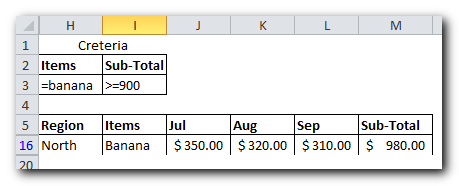
For example, to filter only Banana items, use the following criteria: =”banana”. In Microsoft Excel, it will show =banana in the cell, but you can see the full expression in the formula bar.
As you can see in the screenshot above, the criteria =”=banana” shows only the Banana records with Sub-total greater than or equal to 900, ignoring Green banana and Gold finger banana.
Note. When filtering numeric values that are exactly equal to a given value, you may or may not use the equal sign in the criteria. For instance, to filter records with subtotal equal to 900, you can utilize any of the following Sub-total criteria: =”=900″, =900 or simply 900.
Example 2. Filter text values that begin with a specific character(s)
To display all cells whose contents begin with a specified text, just type that text in the criteria range without the equal sign or double quotes.
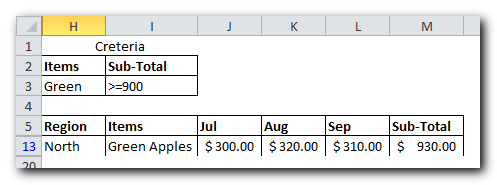
For example, to filter all “green” items with subtotal greater than or equal to 900, use the following criteria:
- Item: Green
- Sub-total: >=900
Excel Advanced Filter with wildcards
To filter text records that partially match, you can use these wildcard characters in the Advanced Filter criteria:
- Question mark (?): Matches any single character.
- Asterisk (*): Matches any group of characters.
- Tilde (~): When followed by *, ?, or ~, it filters cells that contain an actual question mark, asterisk, or tilde.
The table below shows some examples of criteria ranges using wildcards
Criteria | Description | Example |
*text* | Filter cells that contain “text”. | *banana* finds all cells containing the word “banana”, e.g. “green bananas”. |
??text | Filter cells whose contents begin with any two characters, followed by “text”. | ??banana finds cells containing the word “banana” preceded with any 2 characters, like “1#banana” or “//banana”. |
text*text | Filter cells that begin with “text” AND contain a second occurrence of “text” anywhere in the cell. | banana*banana finds cells that begin with the word “banana” and contain another occurrence of “banana” further in the text, e.g. “banana green vs. banana yellow”. |
=”=text*text” | Filter cells that begin with AND end with “text”. | =”=banana*banana” finds cells that begin and end with the word “banana”, e.g. “banana, tasty banana”. |
=”=text1?text2″ | Filter cells that begin with “text1”, end with “text2”, and contain exactly one character in between. | =”=banana?orange” finds cells that begin the word “banana”, end with the word “orange” and contain any single character in between, e.g. “banana/orange” or “banana*orange”. |
text~** | Filter cells that begin with “text”, followed by *, followed by any other character(s). | banana~** finds cells that begin with “banana” followed by asterisk, followed any other text, like “banana*green” or “banana*yellow”. |
=”=?????” | Filters cells with text values that contain exactly 5 characters. | =”=?????” finds cells with any text containing exactly 5 characters, like “apple” or “lemon”. |
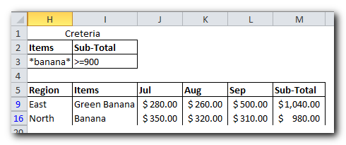
And here is the simplest wildcard criteria in action (*banana*), which finds all cells containing the word “banana”:
Formulas in the Advanced Filter criteria
To create an advanced filter with more complex conditions, you can use one or more Excel functions in the criteria range. To make sure the formula works correctly, follow these rules:
- The formula must give a result of either TRUE or FALSE.
- The criteria range should have at least 2 cells: one for the formula and one for the heading.
- The heading cell for the formula should be blank or should have a different name from any heading in the list range.
- To evaluate the formula for each row of data in the list, use a relative reference (without the $ sign, like A1) to point to the cell in the first row of data.
- To evaluate the formula for just one specific cell or range, use an absolute reference (with the $ sign, like $A$1) to point to that cell or range.
- Always use absolute cell references when referencing the list range in the formula.
For example, to filter rows where sales in August (column C) are greater than sales in July (column D), use the criteria =D5>C5, where 5 refers to the first row of data.
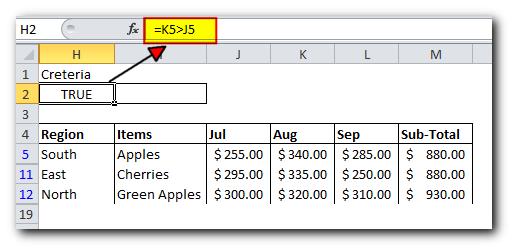
Note. If your criteria includes just one formula like in this example, be sure to include at least 2 cells in the criteria range (formula cell and heading cell).
Using Advanced Filter with AND vs. OR logic
As mentioned at the beginning of this tutorial, the Excel Advanced Filter can use both AND and OR logic, depending on how you set up the criteria range:
- Criteria on the same row are connected with an AND operator (all conditions must be true).
- Criteria on different rows are connected with an OR operator (any one of the conditions can be true).
To help you understand better, let’s look at the following examples
Excel Advanced Filter with AND logic
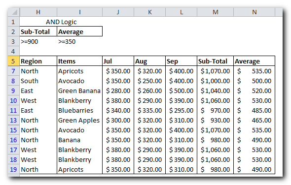
To display records with Sub-total >=900 AND Average >=350, define both criteria on the same row:
Excel Advanced Filter with OR logic
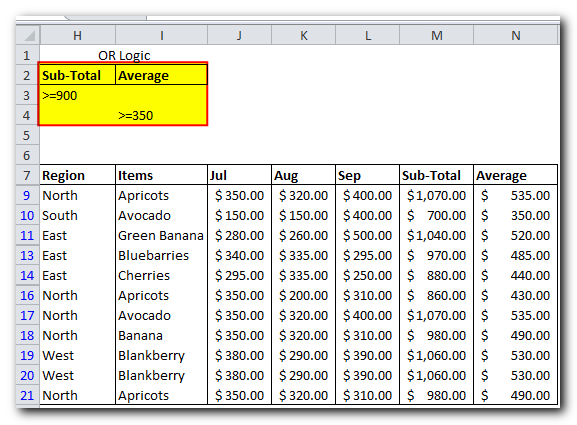
To display records with Sub-total >=900 OR Average >=350, place each condition on a separate row:
Excel Advanced Filter with AND as well as OR logic
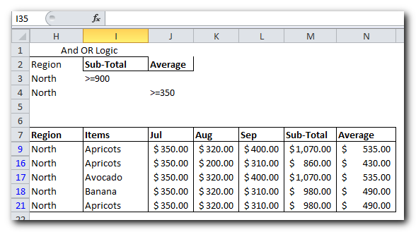
To display records for the North region with Sub-total greater than or equal to 900 OR Average greater than or equal to 350, set up the criteria range in this way:
In other words, the criteria range in this example means:
(Region = North AND Sub-total >= 900) OR (Region = North AND Average >= 350)
Note: The source table in this example has only four regions: North, South, East, and West. So, it’s safe to use ‘North’ in the criteria range. If there were other regions with ‘north’ in their names, like Northwest or Northeast, we would use the exact match criteria: =”North”.
How to extract only specific columns
When setting up the Advanced Filter to copy the results to another location, you can choose which columns to extract.
Before applying the filter, type or copy the headings of the columns you want to extract into the first row of the destination range. For example, if you want to copy the data summary for Region, Item, and Sub-total, type these three column labels in cells H1 to J1 (see the screenshot below).
Next, apply the Excel Advanced Filter and select the ‘Copy to another location’ option under Action. In the ‘Copy to’ box, enter the reference for the column labels in the destination range (H1), and then click OK.
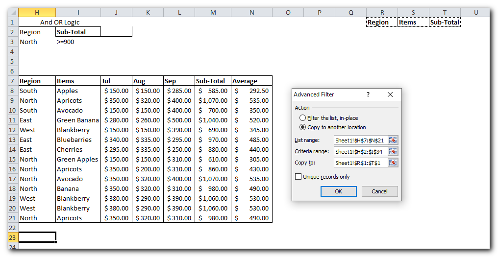
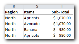
As the result, Excel has filtered the rows according to the conditions listed in the criteria range (North region items with Sub-total >=900), and copied the 3 columns to the specified location:
How to copy filtered rows to another worksheet
If you open the Advanced Filter tool in the worksheet with your original data and choose the ‘Copy to another location’ option while trying to select a range in another sheet, you will see this error message: ‘You can only copy filtered data to the active sheet.’
But there is a way to copy filtered rows to another worksheet! The trick is to start the Advanced Filter from the destination sheet, making it the active sheet.
For example, if your original table is in Sheet1 and you want to copy the filtered data to Sheet2, here’s an easy way to do it:
First, set up the criteria range on Sheet1.
Next, go to Sheet2 and select any empty cell in an unused area of the worksheet.
Now, run Excel’s Advanced Filter by going to the Data tab and clicking on Advanced.
In the Advanced Filter dialog box, select these options:
- Under Action, choose ‘Copy to another location.’
- Click in the List Range box, switch to Sheet1, and select the table you want to filter.
- Click in the Criteria Range box, switch back to Sheet1, and select the criteria range.
- Click in the Copy to box, and select the upper-left cell of where you want to paste the data on Sheet2. (If you only want to copy some columns, type the desired column headings on Sheet2 first, then select those headings.)
- Click OK.
This is how you use the Advanced Filter in Excel. In the next tutorial, we will look at more complex examples of criteria ranges using formulas, so stay tuned!


