Absolute Value in Excel – Simple steps with 4 examples
What is Absolute Value in Excel?
The absolute value of a number is its distance from zero on the number line, regardless of direction, so it’s always a non-negative number. The ABS function in Excel is used to calculate the absolute value in excel of a number.
In other words: the ABS function removes the minus sign (-) from a negative number, making it positive.
- Syntax : =ABS(number)
- number: This is the value you want the absolute value for. It can be a specific number, a cell reference, or a formula.
Examples:
=ABS(-10)will return10.=ABS(10)will return10
The ABS function is useful when you want to ensure that all values are treated as positive, such as in financial models or calculations where negative values aren’t meaningful.
Example 1:- Find Absolute Value in Excel Using ABS Function to
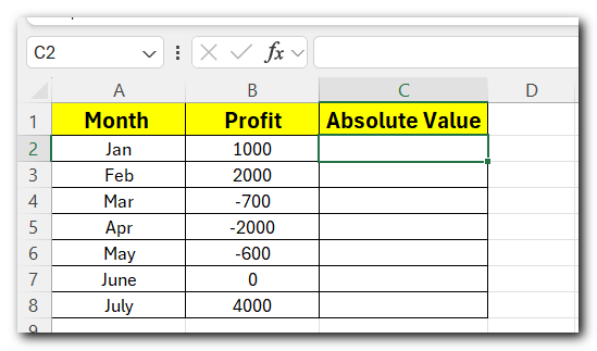
The sample dataset highlights a store’s profit during the first six months of 2023.
To get the absolute results in this dataset:
- Add a column: Absolute Value.
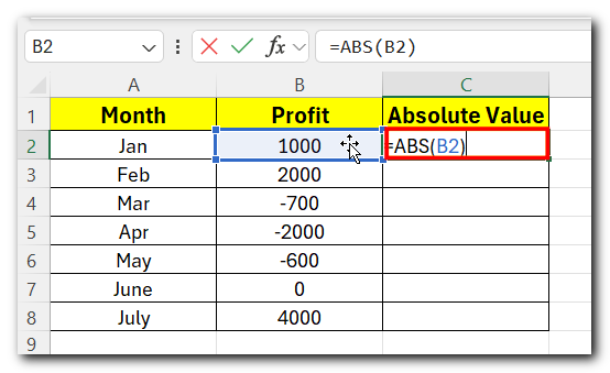
- Enter the ABS function in C2. The formula is:
- =ABS(B2)
- Press Enter and the value of C1 cell will change into absolute value (positive number)
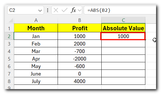
Drag the Fill Handle down to apply the formula to the rest of the cells and see the results.
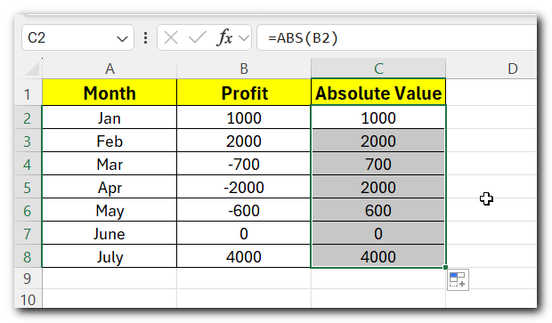
- All the results will be positive when using the ABS function. It only changes negative numbers to positive ones. Positive numbers and zeros stay the same.
Example 2:- Sum absolute values in Excel
To find the absolute sum of all numbers in a range, you can use one of these formulas:
In the first case, you use an array formula to make the SUM function add all the numbers in the specified range.
- For an array formula, use: =SUM(ABS(range))
- After entering the formula, press Ctrl + Shift + Enter to calculate the sum of the absolute values in the specified range.
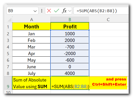
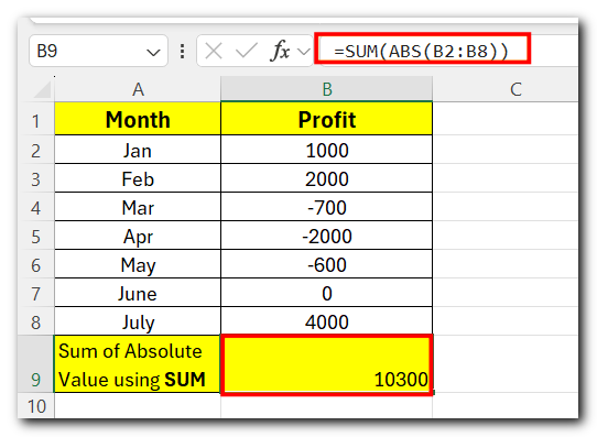
- you will find the result.
- In the second case SUMPRODUCT is naturally an array function and can handle a range without any extra steps.
- For Regular formula use: =SUMPRODUCT(ABS(A2:B5))
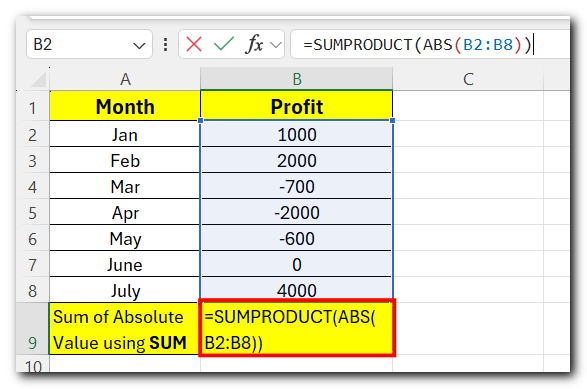
- Regular formula, completed with a standard Enter key press.
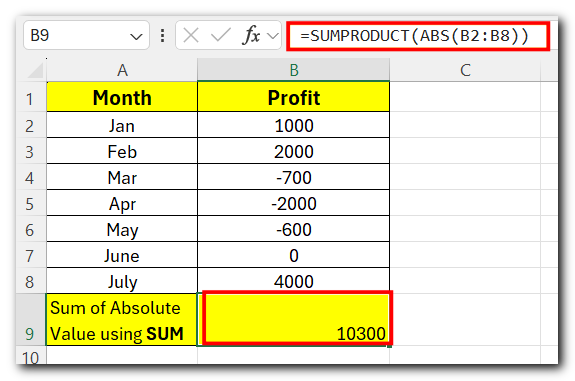
Example 3:- Find the maximum/minimum absolute value in Excel
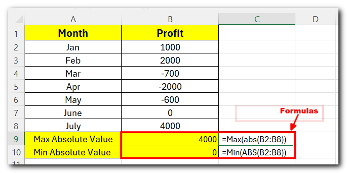
The simplest way to find the minimum and maximum absolute values in Excel is by using these array formulas:
- Maximum absolute value: “MAX(ABS(range))”
- Minimum absolute value: “MIN(ABS(range))”
- To get the max absolute value:
=MAX(ABS(B2:B8)) - To get the min absolute value:
=MIN(ABS(B2:B8))
Remember to complete the array formulas by pressing Ctrl+Shift+Enter.
Example 4:- Average Absolute values in Excel
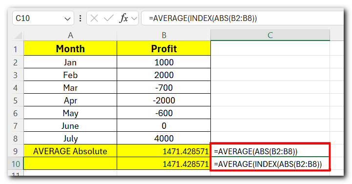
Array formula: =AVERAGE(ABS(range))
Regular formula: =AVERAGE(INDEX(ABS(range),0,0))
For the sample data in cell B9 and B10 use these formulas:
Array formula to average absolute values (press Ctrl + Shift + Enter): =AVERAGE(ABS(B2:B8))
Regular formula to average absolute values: =AVERAGE(INDEX(ABS(B2:B8),0,0))
Conclusion:-
That’s how to do absolute value in Excel by using the ABS function. The formulas discussed in this tutorial are very straightforward and you will hardly have any difficulties adjusting them for your worksheets.
To have a closer look, you’re welcome to learn more Excel Functions


