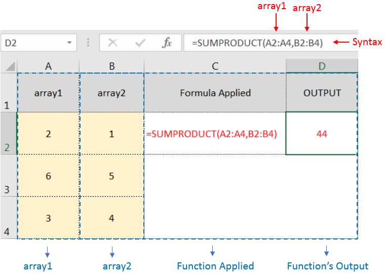
SUMPRODUCT function performs multiplication of numbers within arrays and then sum the values
=SUMPRODUCT(array1,[array2],...
array1 argument is used to give range for which you want to multiply and then sum
[array2] is optional argument and is used to give another range for which you want to multiply and then sum
… means, we can add multiple range by separating them with comma ( , )

SUMPRODUCT Function will first multiply the values within arrays i.e. 1st value of 1st array, multiply with 1st value of 2nd array (2*1=2)
+ 2nd value of 1st array, multiply with 2nd value of 2nd array (6*5=30)
+ 3rd value of 1st array, multiply with 3rd value of 2nd array (3*4=12)
and then, Sum all the values i.e. 2+30+12=44
i.e. =A2*B2 + A3*B3 + A4*B4 = 44
– If function has only one array (i.e. range) then it will Sum all the values
– Multiple ranges can be applied in function by separating them with comma ( , )
– Text/ Blank values will be considered as zero (i.e. 0)
– If No values in range is provided in array argument, then output will return as 0 (zero)
Hope you learnt this Function,
Don’t forget to leave your valuable comments!
If you liked this article and want to learn more similar tricks, please Subscribe us or follow us on Social Media by clicking below buttons:

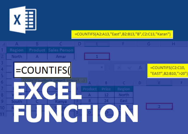
COUNTIFS function is used to get the total count for number of times the various criteria across ranges are met.

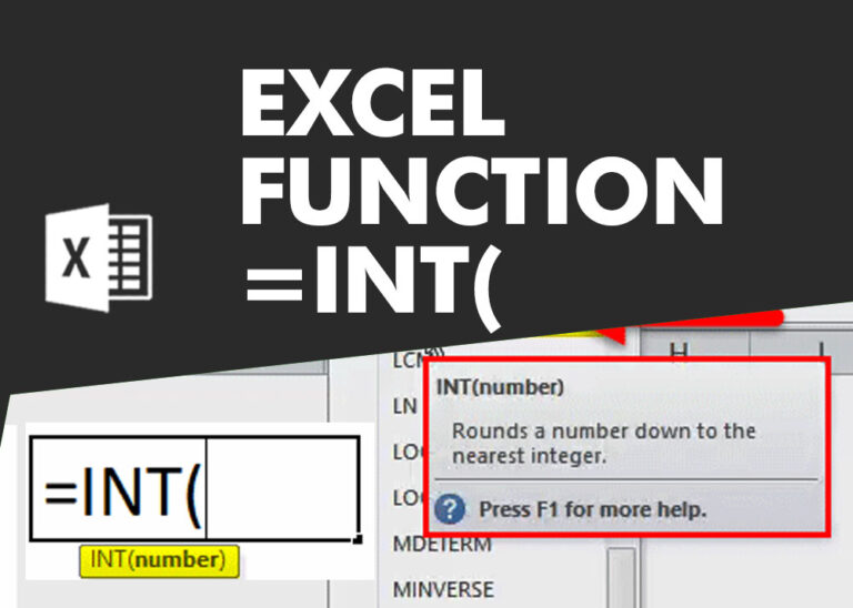
INT function is used to round down the numeric value to nearest integer. INT Function has one required argument i.e. number.

Table of Content Introduction Benefits of Using Outlook and Excel for Work Allocation Setting Up Your Outlook-Based Excel Tool Managing Work Allocation Conclusion Download Free Excel Template Introduction Efficient work allocation is crucial for organizations…

This video will help you to understand how you may use conditional formatting to highlight row based on conditions. Subscribe us for more updates

This tutorial shows you three easy ways to add hyperlinks in Excel. You will learn how to insert, change, and remove hyperlinks in your worksheets. It also explains how to fix links that don’t work.
Hyperlinks are often used on the internet to move between websites. In Excel, you can create links like that too. You can make a link to another cell, a different sheet, or even another workbook. You can also link to open a new Excel file or start an email message. This guide will show you how to do all of this in Excel 2016, 2013, 2010, and older versions.

MID function is used for extracting the mid characters from the available string. The output of the function returns the extracted characters in new cell.