We can place multiple criteria or conditions in function by separating them with comma ( , )
=COUNTIFS(criteria_range1, criteria1, [criteria_range2, criteria2]…)
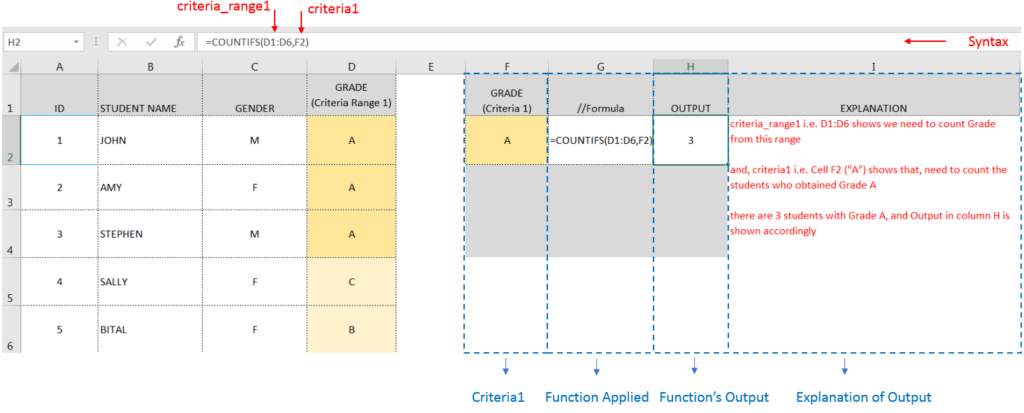
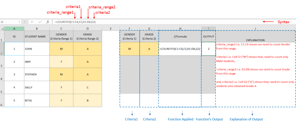
criteria_range1 argument is used to give the range in which criteria1 needs to find
criteria1 argument is used to give criteria for count. We can give value (example “A”, >10, 50) or cell reference# (example: F2) in this argument
[criteria_range2] optional argument is used to give the ANOTHER range in which criteria2 needs to find
[criteria2] optional argument is used to give criteria2 for count. Value or cell reference# can be given.
Kindly note, we can add multiple criteria in the function by separating them with Comma ( , )
Here, we want to get the count of students who obtained Grade A:
We will be using COUNTIFS function as follows:

Here, we want to get the count of Male Students (criteria1) who have obtained Grade A (criteria2):
We will be using COUNTIFS function as follows:

Hope you learnt this Function,
Don’t forget to leave your valuable comments!

AVERAGE function is used to get the average of numbers. Function applies formula i.e. average = Sum of all values / (Divided by) number of items.

Watch: How to use WEEKNUM Function in Excel? What is WEEKNUM Function? The WEEKNUM function in Excel returns the week number of a given date. It is a DATE and TIME function that can be…

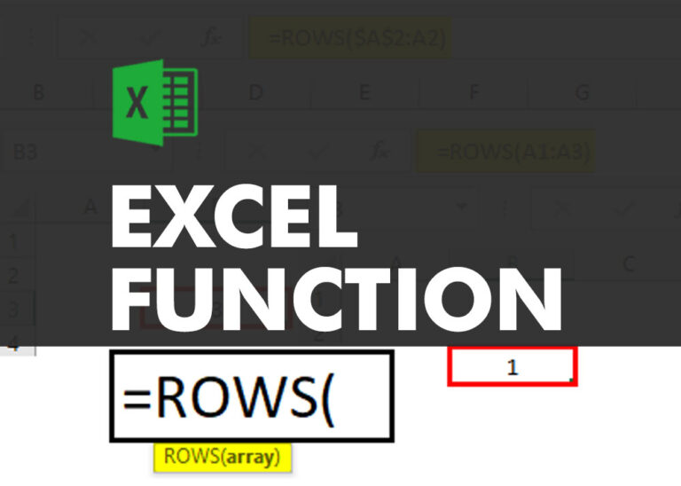
ROWS function is used to get the total count of rows in an array or in cells range in an excel worksheet.

In this tutorial, we’re going to explore one of the most intriguing features in Excel: the OFFSET function.
So, what is the OFFSET function in Excel? Simply put, OFFSET gives you a reference to a range of cells that’s moved from a starting point by a certain number of rows and columns.

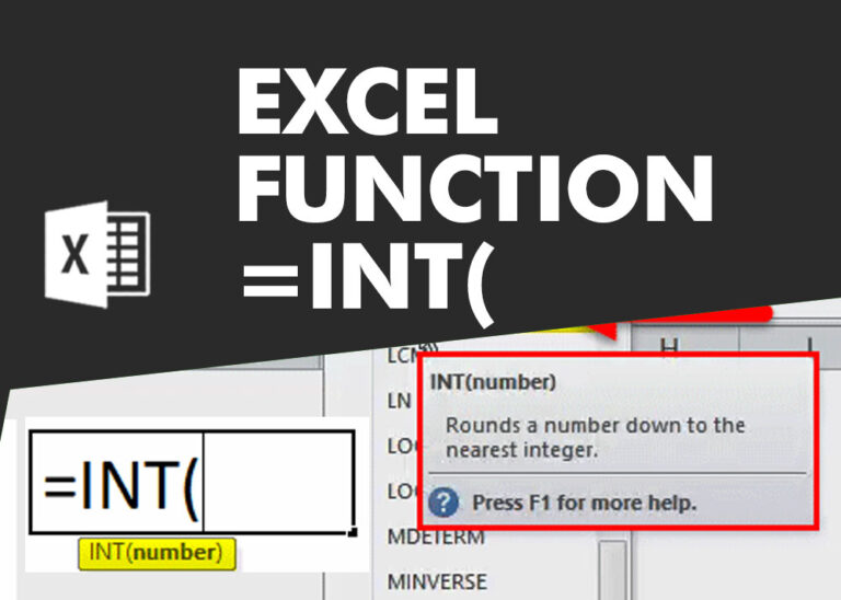
INT function is used to round down the numeric value to nearest integer. INT Function has one required argument i.e. number.

LARGE function is used to get the Largest k-th value from the range.
LARGE Function has two required arguments i.e. array, and k