=LOWER(text)
text argument, is used to give the cell reference of the string or value that needs to be changed to Lower Case
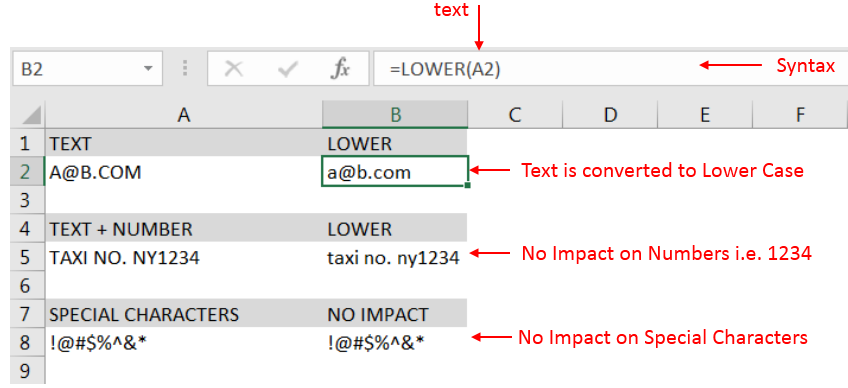
Here we have some examples where in “Column A” various type of strings are available and are required to be changed to “LOWER CASE”. Output of the function returns value in ”Column B” and explanation is also provided.
text argument, “A2” is the cell reference for text that is to be changed to “LOWER CASE”

– Output in Cell “B2” is showing that the string is changed to Lower Case.
– Output in Cell “B5” is including text and number and no impact in “Numbers” are shown.
– Output in Cell “B8” has only Special Characters and there is no impact of “LOWER Case” function.
– Number/ Punctuation/ Space/ Special Characters will not have any impact of Function
– If cell reference is not correctly provided in the function, then it will give output as “#VALUE!” (Error)
– Function should give output in “General” format, however if output is not as per the desired format then we need to change the cell format to “GENERAL”
Hope you learnt this Function,
Don’t forget to leave your valuable comments!
If you liked this article and want to learn more similar tricks, please Subscribe to us.

LEFT function is used for extracting the “Left Most” characters from the available string. The output of the function returns the extracted characters in new cell

Few Excel Tips 1. CHANGE DIRECTION WHEN YOU PRESS ENTER Whenever you press enter, you must be thinking why my cell selection shifts down. Why it can’t go UP, Down, Left. Surprised This is very…

This step-by-step tutorial empowers you to leverage Power Query’s robust filtering capabilities. Learn to filter by date, text, numbers, and more, streamlining your workflow and unlocking deeper insights from your data. Watch now and elevate your Excel expertise!

This article unveils the magic of Power Query, a built-in Excel tool that simplifies data organization. Learn how to sort by single or multiple columns, create layered sorts for complex needs, and even reverse your data order entirely. Power Query puts you in control, transforming your data into a well-structured format for effortless analysis.

The tutorial demonstrates how to find a date any number of days before or after today, counting either all days or only business days.

How to count words in Excel using the LEN function along with other Excel functions. It also gives formulas for counting words or text, whether case-sensitive or not, in a cell or range.