Linear regression analysis in Excel
The tutorial teaches you the basics of regression analysis and shows a few ways to do linear regression in Excel.
Imagine this: you have a lot of data and need to predict next year’s sales for your company. You’ve found many factors that could affect the sales, maybe even hundreds. But how do you know which ones really matter? You can use regression analysis in Excel. It will help answer this and other questions, like: Which factors are important and which ones don’t matter? How connected are these factors? And how confident can you be in your predictions?”
Does this work better for you?
Table of Contents
Regression analysis in Excel - the basics
In statistical modeling, regression analysis is used to estimate the relationships between two or more variables:
Dependent variable (aka criterion variable) is the main factor you are trying to understand and predict.
Independent variables (aka explanatoryvariables, or predictors) are the factors that might influence the dependent variable.
Regression analysis helps you see how the dependent variable changes when one of the independent variables changes, and it helps you figure out, using math, which variables really make a difference.
Technically, regression analysis uses something called the sum of squares, which is a way to measure how spread out the data points are. The goal is to make the sum of squares as small as possible and draw a line that fits the data as closely as it can.
In statistics, there are two types of linear regression: simple and multiple. Simple linear regression looks at the relationship between one dependent variable and one independent variable using a straight line. If you use two or more independent variables to predict the dependent variable, it’s called multiple linear regression. If the relationship doesn’t follow a straight line, you use nonlinear regression instead. This tutorial will focus on simple linear regression
Linear regression equation
Mathematically, a linear regression is defined by this equation:
y = bx + a + ε
Where:
- x is an independent variable.
- y is a dependent variable.
- a is the Y-intercept, which is the expected mean value of y when all x variables are equal to 0. On a regression graph, it’s the point where the line crosses the Y axis.
- b is the slope of a regression line, which is the rate of change for y as x
ε is the random error term, which is the difference between the actual value of a dependent variable and its predicted value.
The linear regression equation always includes an error term because, in real life, predictions are never 100% accurate. However, some programs, like Excel, handle the error term for you in the background. In Excel, you use the least squares method for linear regression, trying to find the values of ‘a’ and ‘b’ so that
y = bx + a
For our example, the linear regression equation takes the following shape:
Umbrellas sold = b * rainfall + a
There exist a handful of different ways to find a and b. The three main methods to perform linear regression analysis in Excel are:
- Regression tool included with Analysis ToolPak
- Scatter chart with a trendline
- Linear regression formula
Below you will find the detailed instructions on using each method.
How to do linear regression in Excel with Analysis ToolPak
This example shows how to run regression in Excel by using a special tool included with the Analysis ToolPak add-in.
Enable the Analysis ToolPak add-in
Analysis ToolPak is available in all versions of Excel 365 to 2003 but is not enabled by default. So, you need to turn it on manually. Here’s how:
- In your Excel, click File> Options.
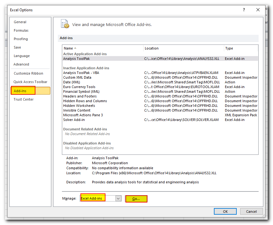
- In the Excel Optionsdialog box, select Add-ins on the left sidebar, make sure Excel Add-ins is selected in the Manage box, and click Go.
In the Add-ins dialog box, tick off Analysis Toolpak, and click OK:
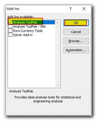
This will add the Data Analysis tools to the Data tab of your Excel ribbon
Run regression analysis
In this example, we will do a simple linear regression in Excel. We have a list of average monthly rainfall for the past 24 months in column B, which is our independent variable (the predictor), and the number of umbrellas sold in column C, which is the dependent variable. While many other factors can affect sales, for now, we will focus only on these two variables
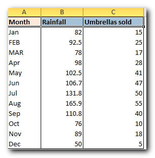
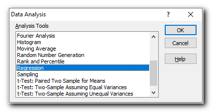
Once the Analysis Toolpak is enabled, follow these steps to do regression analysis in Excel:
- Go to the Data tab.
- In the Analysis group, click the Data Analysis button.

Select Regression and click OK.
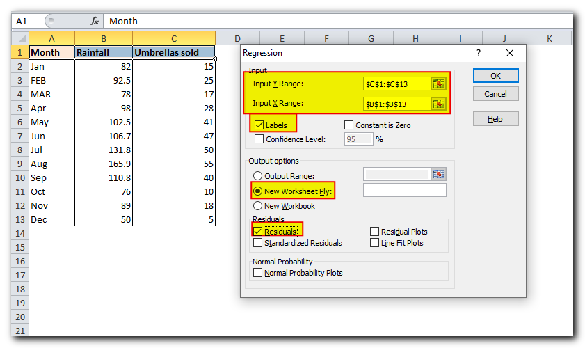
In the Regression dialog box, set the following:
- Select the Input Y Range, which is your dependent variable. In our case, this is the umbrella sales (C1).
- Select the Input X Range, which is your independent variable. For this example, it’s the average monthly rainfall (B1).
- If you are doing multiple regression with more variables, select two or more columns with different independent variables.
- Check the Labels box if your X and Y ranges have headers at the top.
- Choose where you want the results to appear, like in a new worksheet.
If you want to see the difference between predicted and actual values, check the Residuals box.
Click OK and observe the regression analysis output created by Excel.
Interpret regression analysis output
As you’ve just seen, doing regression in Excel is easy because all the calculations are done automatically. Understanding the results is a bit harder because you need to know what each number means. Below is a breakdown of the 4 main parts of the regression analysis output.
Regression analysis output: Summary Output
This part tells you how well the calculated linear regression equation fits your source data.
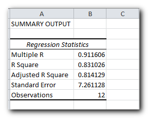
Here’s what each part means:
Multiple R: This is the Correlation Coefficient, which shows how strong the relationship is between two variables. The value can be between -1 and 1. The closer the value is to either -1 or 1, the stronger the relationship
- 1 means a strong positive relationship
- -1 means a strong negative relationship
- 0 means no relationship at all
R Square: This is the Coefficient of Determination, which shows how well the data fits the regression line. It tells you what percentage of the data points are close to the line. The R² value is calculated from the total sum of squares, which measures how far the data is from the average.
In our example, R² is 0.83 (rounded to two digits), which is pretty good. This means 83% of our data fits the regression model. In other words, 83% of the changes in the dependent variable (y-values) are explained by the independent variable (x-values). Usually, an R² value of 95% or more is considered a good fit.
Adjusted R Square: This is the R Square value adjusted for the number of independent variables in the model. You should use this value instead of R Square when doing multiple regression analysis.
Standard Error: This is another measure of how well your model fits the data. It shows how precise your regression is—the smaller the number, the more accurate your equation. While R Square shows the percentage of variation explained by the model, Standard Error tells you the average distance between the data points and the regression line.
Observations: This is simply the number of data points used in your model.
Regression analysis output: ANOVA
The second part of the output is Analysis of Variance (ANOVA):

Basically, it splits the sum of squares into individual components that give information about the levels of variability within your regression model:
- df is the number of the degrees of freedom associated with the sources of variance.
- SS is the sum of squares. The smaller the Residual SS compared with the Total SS, the better your model fits the data.
- MS is the mean square.
- F is the F statistic or F-test for the null hypothesis. It is used to test the overall significance of the model.
- Significance F is the P-value of F.
The ANOVA part is rarely used for a simple linear regression analysis in Excel, but you should definitely have a close look at the last component. The Significance F value gives an idea of how reliable (statistically significant) your results are. If Significance F is less than 0.05 (5%), your model is OK. If it is greater than 0.05, you’d probably better choose another independent variable.
Regression analysis output: coefficients
This section provides specific information about the components of your analysis

The most useful component in this section is Coefficients. It enables you to build a linear regression equation in Excel:
y = bx + a
For our data set, where y is the number of umbrellas sold and x is an average monthly rainfall, our linear regression formula goes as follows:
Y = Rainfall Coefficient * x + Intercept
Equipped with a and b values rounded to three decimal places, it turns into:
Y=0.45*x-19.074
or example, with the average monthly rainfall equal to 82 mm, the umbrella sales would be approximately 17.8:
0.45*82-19.074=17.8
n a similar manner, you can find out how many umbrellas are going to be sold with any other monthly rainfall (x variable) you specify.
Regression analysis output: residuals
If you compare the estimated and actual number of umbrellas sold for a month with 82 mm of rainfall, you’ll notice they are slightly different:
- Estimated: 20.6 (calculated earlier)
- Actual: 15 (from row 5 of the data)
Why is there a difference? Because independent variables (like rainfall) are never perfect at predicting dependent variables (like umbrella sales). The residuals can show you how far off the actual values are from the predicted values.
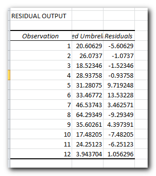
For the first data point (rainfall of 82 mm), the residual is approximately -5.6. So, we add this number to the predicted value, and get the actual value: 20.6 – 5.6 = 15
How to make a linear regression graph in Excel
If you need to quickly visualize the relationship between the two variables, draw a linear regression chart. That’s very easy! Here’s how:
- Select the two columns with your data, including headers.
- On the Insettab, in the Chats group, click the Scatter chart icon, and select the Scatter thumbnail (the first one):
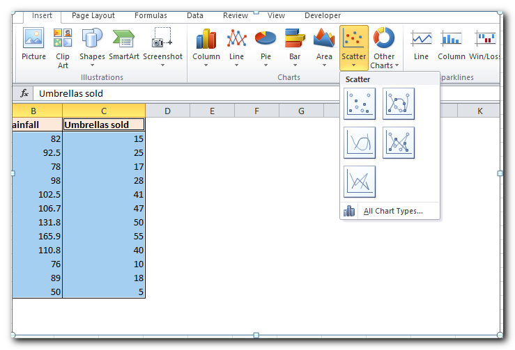
This will insert a scatter plot in your worksheet, which will resemble this one:
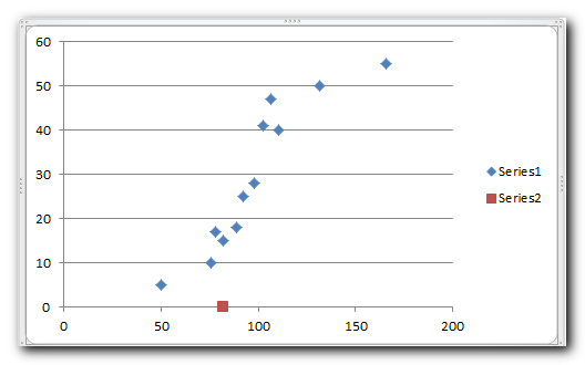
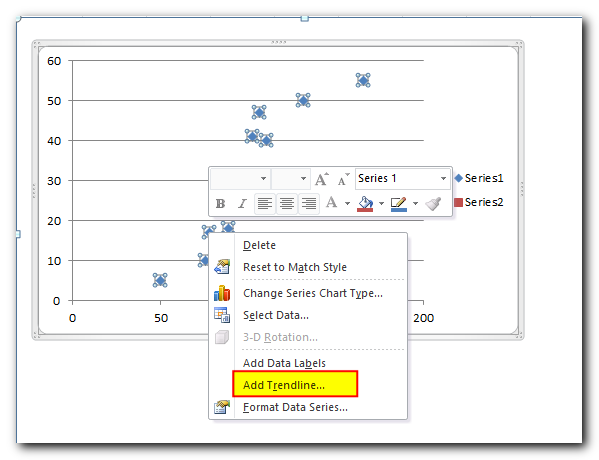
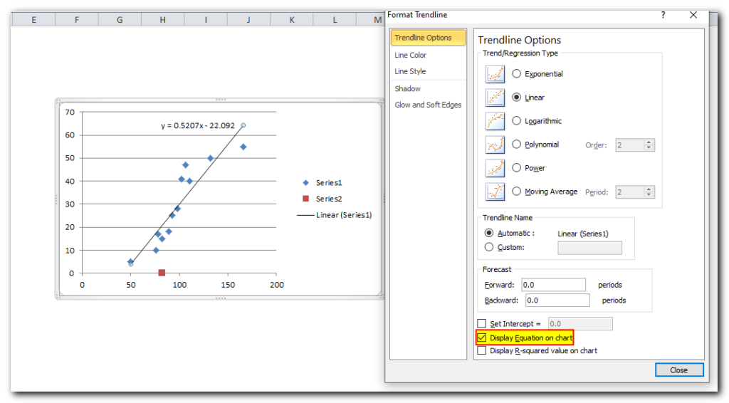
Now, we need to draw the least squares regression line. To have it done, right click on any point and choose Add Trendline… from the context menu
On the right pane, select the Linear trendline shape and, optionally, check Display Equation on Chart to get your regression formula:
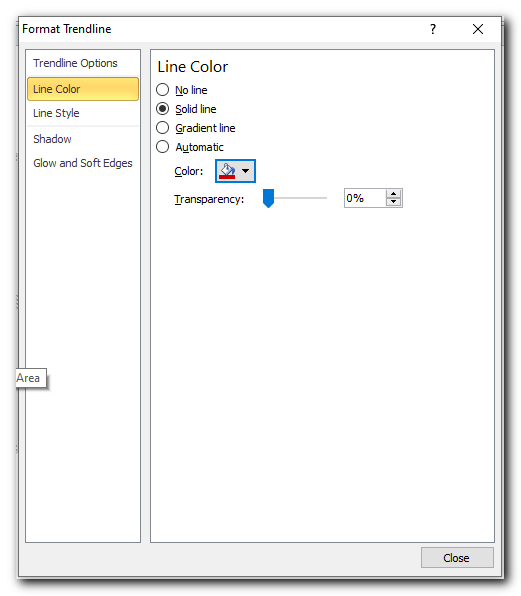
Switch to the Fill & Line tab and customize the line to your liking. For example, you can choose a different line color and use a solid line instead of a dashed line (select Solid line in the Dash type box):
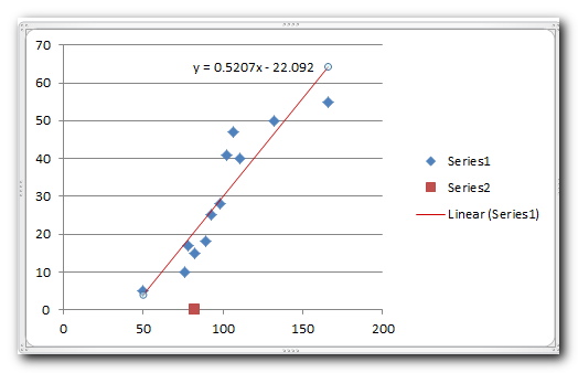
At this point, your chart already looks like a decent regression graph:
You might still want to make a few more changes:
- Move the equation to where it looks best.
- Add titles to the axes (go to the Chart Elements button and choose Axis Titles).
- If your data points start in the middle of the chart, you might notice extra white space. To fix this, you can change the axis scale to remove the white space.
Here’s what the improved regression graph looks like
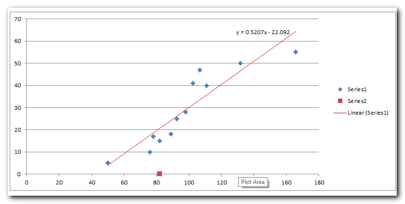
Important note! In a regression graph, the independent variable should always be on the X-axis (horizontal) and the dependent variable on the Y-axis (vertical). If your graph is plotted the wrong way, swap the columns in your worksheet and create the chart again. If you can’t change the data in your worksheet, you can switch the X and Y axes directly in the chart.
How to do regression in Excel using formulas
Microsoft Excel has a few statistical functions that can help you to do linear regression analysis such as LINEST, SLOPE, INTERCEPT, and CORREL.
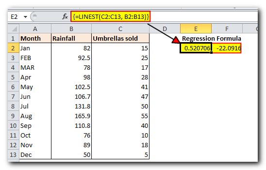
The LINEST function uses a method called least squares regression to find the straight line that best fits your data. It returns a set of values that describe that line. You can learn more about how the function works in this tutorial. For now, let’s create a formula for our sample data:
=LINEST(C2:C25, B2:B25)
Because the LINEST function returns an array of values, you must enter it as an array formula. Select two adjacent cells in the same row, E2:F2 in our case, type the formula, and press Ctrl + Shift + Enter (Array Function) to complete it.
The formula returns the b coefficient (E1) and the a constant (F1) for the already familiar linear regression equation:
y = bx + a
If you avoid using array formulas in your worksheets, you can calculate a and b individually with regular formulas:
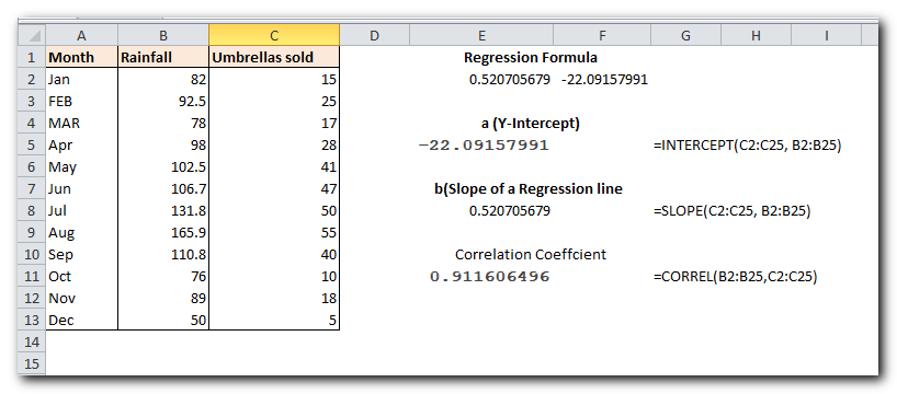
Get the Y-intercept (a):
=INTERCEPT(C2:C25, B2:B25)
Get the slope (b):
=SLOPE(C2:C25, B2:B25)
Additionally, you can find the correlation coefficient (Multiple R in the regression analysis summary output) that indicates how strongly the two variables are related to each other:
=CORREL(B2:B25,C2:C25)
The following screenshot shows all these Excel regression formulas in action:
Tip. If you’d like to get additional statistics for your regression analysis, use the LINEST function with the stats parameter set to TRUE as shown in this example.
That’s how you perform linear regression in Excel. However, remember that Microsoft Excel is not a specialized statistical tool. If you need to do more advanced regression analysis, you might want to use software like XLSTAT or RegressIt.
To explore the formulas and techniques we’ve discussed, feel free to download our sample workbook below. Thank you for reading!


