How to use Transpose Function in excel
This tutorial explains how the TRANSPOSE function works and shows you the right way to use it to switch data in Excel.
Everyone has different preferences, even for work habits. Some people like to arrange data in vertical columns, while others prefer horizontal rows. If you ever need to switch the direction of your data quickly, the TRANSPOSE function can help
Table of Contents
Excel TRANSPOSE function - syntax
The TRANSPOSE function in Excel is used to change rows into columns, or columns into rows. It helps you switch the direction of a selected range from horizontal to vertical, or the other way around.
The function only needs one input:
TRANSPOSE(array)
An array is the group of cells you want to switch.
When transposed, the first row of the original group becomes the first column in the new group, the second row becomes the second column, and so on.
Important note! For the TRANSPOSE function to work in Excel 2019 and lower, you must enter it as an array formula by pressing Ctrl + Shift + Enter. In Excel 2021 and Excel 365 that support arrays natively, it can be entered as a regular formula.
How to use the TRANSPOSE function in Excel
The TRANSPOSE function’s syntax is clear and hard to get wrong when creating a formula. The tricky part is entering it correctly into the worksheet. If you’re not very experienced with Excel formulas, especially array formulas, be sure to follow the steps below carefully.
Count the number of columns and rows in the original table
For starters, find out how many columns and rows your source table contains. You will need these numbers in the next step.
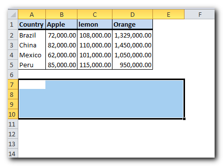
In this example, we are going to transpose the table that shows the volume of fresh fruit exports by county
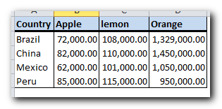
Our source table has 4 columns and 5 rows. Keeping these figures in mind, proceed to the next step.
Select the same number of cells, but change the orientation
Your new table will have the same number of cells but will be flipped from horizontal to vertical, or the other way around. So, you need to select a range of empty cells with the same number of rows as the original table’s columns, and the same number of columns as the original table’s rows.
For example, here we select 5 columns and 4 rows
Type the TRANSPOSE formula
After selecting a range of blank cells, enter the Transpose formula:
=TRANSPOSE(A1)
Follow these steps:
First, type the equal sign, the function name, and an opening parenthesis: =TRANSPOSE(
Next, use the mouse to select the source range or type it in manually
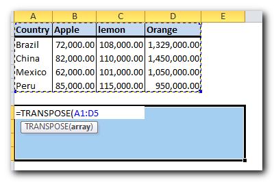
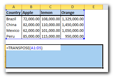
Finally, type the closing parenthesis, but don’t hit the Enter key! At this point, your Excel Transpose formula should look similar to this:
Complete the TRANSPOSE formula
“Press Ctrl + Shift + Enter to complete your array formula correctly. Why is this needed? Because the formula works on multiple cells, which is what array formulas are designed for.
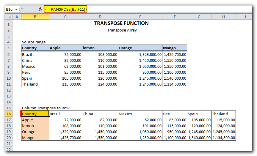
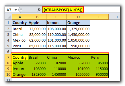
When you press Ctrl + Shift + Enter, Excel will automatically add {curly braces} around your Transpose formula in the formula bar. This shows it’s an array formula. Don’t try to type the curly braces yourself—it won’t work.
The screenshot below shows that our table was successfully flipped, converting 4 columns into 4 rows
How to transpose data in Excel without zeros for blanks
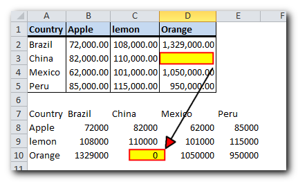
If one or more cells in the original table is empty, those cells will have zero values in the transposed table, as shown in the screenshot below:
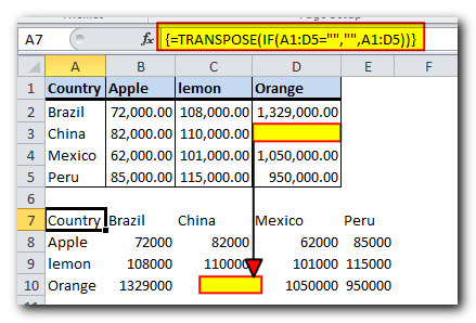
If you wish to return blank cells instead, nest the IF function inside your TRANSPOSE formula to check whether a cell is blank or not. If the cell is blank, IF will return an empty string (“”), otherwise supply the value to transpose:
=TRANSPOSE(IF(A1:D5=””,””,A1:D5))
Enter the formula as explained above (please remember to press Ctrl + Shift + Enter to finish the array formula correctly), and you will have a result similar to this:
Tips and notes on using TRANSPOSE in Excel
As you have just seen, the TRANSPOSE function has a number of quirks that may confuse unexperienced users. The below tips will help you avoid typical mistakes.
1. How to edit a TRANSPOSE formula
Since TRANSPOSE is an array function, you can’t change just part of the result it gives. To edit the Transpose formula, select the entire range the formula covers, make your changes, and press Ctrl + Shift + Enter to save the updated formula.
2. How to delete a TRANSPOSE formula
To remove a Transpose formula from your worksheet, select the whole range referenced in the formula, and press the Delete key.
3. Replace TRANSPOSE formula with values
When you use the TRANSPOSE function to flip a range, the original and new tables are linked. This means if you change something in the original table, the same value will change in the flipped table automatically.
If you want to remove this link, replace the formula with the actual values. To do this, select the transposed values, press Ctrl + C to copy, right-click, and choose Paste Special > Values.
For more details, see How to convert formulas to values. That’s how you use the TRANSPOSE function to rotate data in Excel. Thank you for reading, and I hope to see you on our blog next week!


