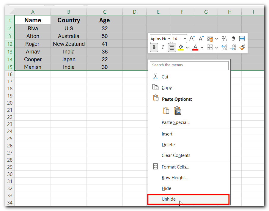
Unhide Cells in Excel – 5 Easy Methods
2. Unhide Cells in Excel using Format Options
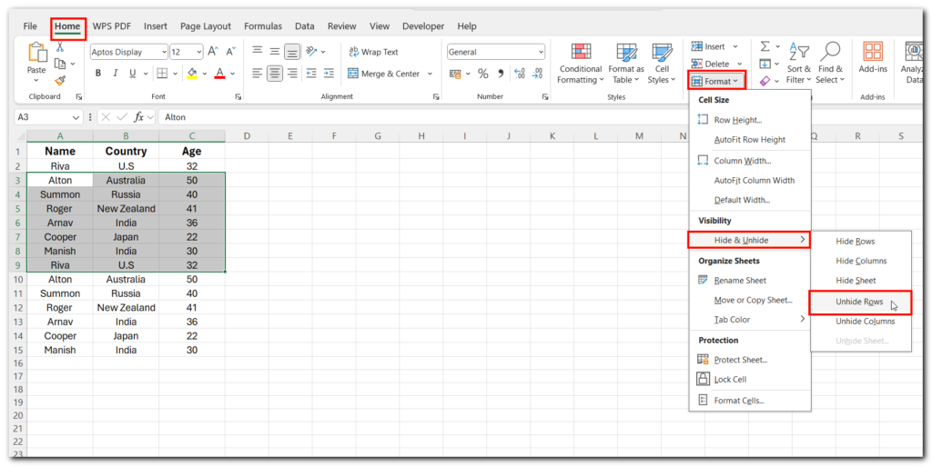
Here’s how you can unhide hidden rows or columns using the Format option:
- Highlight the cells around the hidden ones.
- Go to the Home tab and click Format in the Cells group.
- Under Visibility, choose Hide & Unhide.
- Select Unhide Rows or Unhide Columns to reveal the hidden cells.
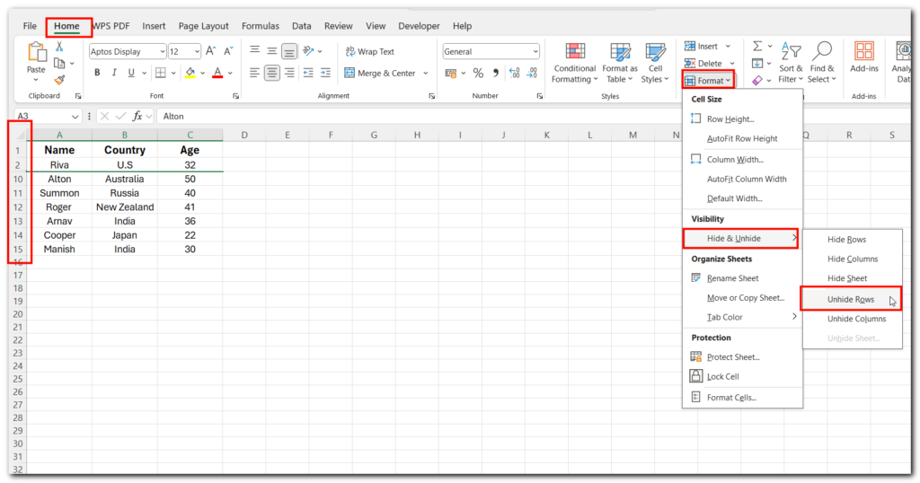
This method works if the regular ‘Unhide’ button doesn’t!
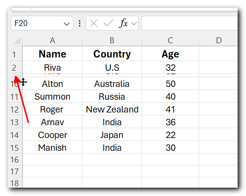
3. Unhide Cells in Excel by Dragging
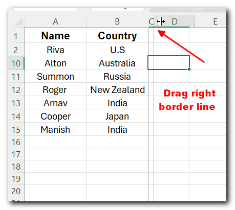
- Double-clicking the right border of a hidden column can automatically adjust its width, but it might make the sheet too wide if many columns are hidden.
- To avoid this, you can drag the column border instead.
- Look for the double-line between two visible columns. This is where the hidden columns are.
- Left-click on the right side of the double-line and drag it to the right until the hidden columns become visible.
4. Shortcut to Unhide Cells in Excel
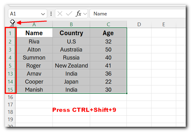
- Unhide Rows: Select the hidden rows and press Ctrl + Shift + 9.
- Unhide Columns: Select the hidden columns and press Ctrl + Shift + 0.
- For Hidden Worksheet : Ctrl + Shift + S
5. Unhide Cells in Excel Using Name Box
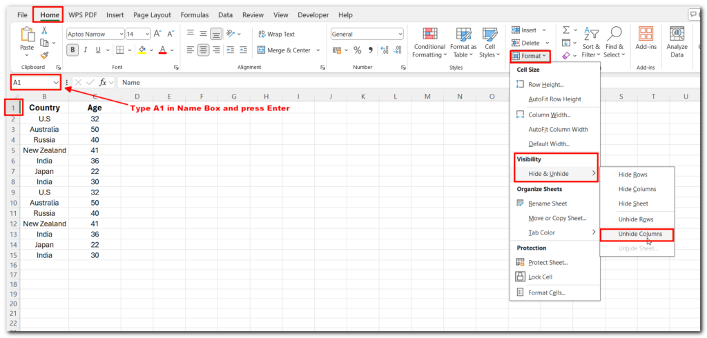
To unhide column A using the Name Box in Excel, follow these steps:
- Click on the Name Box (located to the left of the formula bar).
- Type A1 and press Enter.
- Green line indicates that column A selected (even though it’s hidden), go to the Home tab.
- Click on Format in the Cells group.
- Under Visibility, choose Unhide Columns.
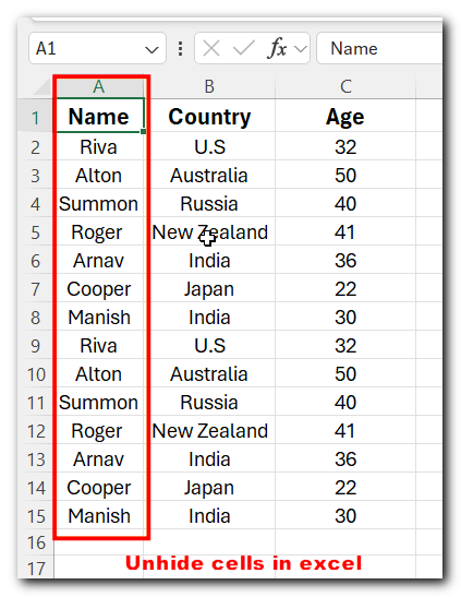
This will unhide column A.
Conclusion
Unhiding cells in Excel is an easy way to make sure you can see and use all your data. Whether rows or columns are hidden, Excel provides simple tools to unhide them, By learning these steps, you can quickly find and manage hidden data, making it easier to work with your spreadsheet and ensuring nothing is missed.
FAQs
- How to Hide Cells in Excel?
- Select the cell(s) you want to hide.
- Go to the Home tab > Cells group > Format > Format Cells.
- In the Format Cells menu, under the Number tab, select Custom.
- Type
;;;(three semicolons) and click OK.
2. How to Hide Gridlines in Excel?
- Go to the Page Layout tab.
- Uncheck the View box under Gridlines.
3. How to Hide Formulas in Excel?
- Select the cells with formulas.
- Go to Format Cells > Protection tab, check Hidden, and click OK.
- Then, go to the Review tab > Protect Sheet. Ensure “Protect worksheet and contents of locked cells” is enabled, and click OK.
4. The first 7 rows of my Excel sheet are missing, and using the “unhide” option from the Format menu isn’t working. How can I fix this?
- You need to unlock the cells first (using the format pop-up), then hide them again before trying to unhide them.
Hope you this article is helpful. Follow us to learn more .
Related articles:-
How to Hide Sheet in Excel with or without VBA?
How to Delete Blank Rows in Excel – 6 Easy Methods
VBA Code to Find Last Column or Row of a Sheet

