Excel Cell Reference – 3 simple ways
What is Excel Cell Reference?
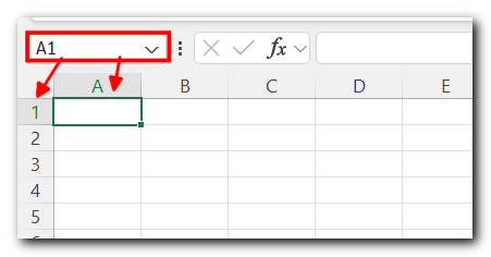
 The letter comes from the column (A, B, C…) and the number comes from the row (1, 2, 3…).
This is how Excel organizes its grid with rows and columns.

- Columns in Excel are labeled with letters, while rows are labeled with numbers.
- A cell is created where a row and column meet, and its name is a mix of the row and column.
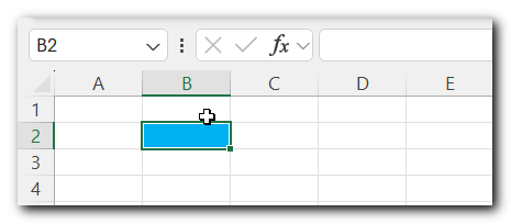
- For example, in the image below, the highlighted cell is at the intersection of Column B and Row 2.

- The highlighted cell is called Cell B2 (where Column B meets Row 2).
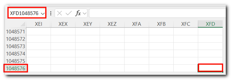
- Similarly, scroll to the end of your worksheet to see that even the last cell, Cell XFD1048576 (Column XFD and Row 1048576), is named in the same way.

- It is created at the intersection of Column XFD and Row 1048576.
You should some Few Simple Excel Tips to improve your excel knowledge.
Types of Excel Cell Reference
1. Relative Cell Reference
2. Absolute Cell Reference
3. Mixed Cell Reference
1. Relative Cell Reference in Excel
- The below image shows the total marks for each subject in Row 3 and marks obtained in Row 4

- Let’s quickly find the percentage in each subject.
- Write the formula in Cell B5 like this: “=B4/B3*100″

- Let’s calculate the marks for the other subjects without writing a formula for each one.
- Simply drag the formula from Cell B5 to the rest of the cells. This will apply the same formula to all of them!

- But what did Excel do?
- When you move formulas across cells, Excel updates the cell references based on the rows and columns
- The formula changes because of relative references. When copied from Column B to Column C, Excel adjusts the cell references to match the new position.
- This way, you don’t need to write a formula for each cell.
- Just create one formula and copy it to the other cells. Excel will automatically adjust the cell references for you. 💪
2. Absolute Cell Reference in Excel
An absolute cell reference means you lock a specific cell in a formula, so it doesn’t change when you copy the formula to other cells. You do this by adding $ symbols

The table shows the marks obtained in various subjects, If we want to calculate the percentage for each subject we will use the formula:-
=B4/B3*100
If you drag the formula to other subject excel will change the reference for the other cells too.

But what if the total marks are always the same? You need to lock the total marks cell using an absolute reference. Here’s how to lock a cell
If total marks are always in cell B3, you can write the formula like this: = B4/$B$3*100

Now, the cell B3 won’t change when you drag the formula, but the marks obtained will.
This makes calculating percentages for all subjects super easy without having to manually adjust the formula!
PROTIP 💡:- Use Absolute Excel cell references when you want a number (like total marks) to stay the same in different calculations.
3. Mixed Cell Reference in Excel
A mixed excel cell reference is when only one part of the cell (either the row or the column) stays fixed, while the other part changes. This is helpful when you want part of your formula to remain the same and the other part to update as you move across the table.
Let’s understand this with the table below:

In a mixed reference, you can lock either the row or the column in a formula:
- $B3: The column is locked (B won’t change), but the row (3) can change.
- B$3: The row is locked (3 won’t change), but the column (B, C etc.) can change.
Lets learn this with the help of example:
step 1: You have total marks in row 2 (B3 to G3) and marks obtained in row 3 (B4 to G4).
Step 2: To calculate percentages in row 4, use this formula in cell B5 = B4/B$3 * 100

Here, B$3 locks the row 2 (total marks), but the column B will change as you move across the subjects.
If you drag the formula from B5 to C5, Excel will adjust it to use the marks obtained for English, but the total marks will always refer to row 3
Protip💡:- Use mixed references when you need part of the cell to stay the same (like total marks) while the other part can change (like marks obtained).
This makes all Excel formulas you use will work easily.


