How to use IFERROR Function in Excel
This tutorial explains how to use IFERROR function in Excel to catch and handle errors. It shows you how to replace errors with a blank cell, a different value, or a custom message. You’ll also learn how to use IFERROR with functions like VLOOKUP and INDEX MATCH, and how it compares to other error-checking functions like IF ISERROR and IFNA
Table of Contents
Excel IFERROR function - syntax and basic uses
The IFERROR function in Excel is made to catch and handle errors in formulas and calculations. Simply put, IFERROR checks a formula, and if the formula results in an error, it gives back a value you choose. If there’s no error, it shows the result of the formula.
The syntax for the IFERROR function in Excel looks like this:
IFERROR(value, value_if_error)
Here’s what each part of the IFERROR function means:
- Value (required) – This is what you want to check for errors. It can be a formula, a value, a cell reference, or an expression.
- Value_if_error (required) – This is what will be shown if an error is found. It can be a blank cell (empty string), a text message, a number, or even another formula.
For example, if you’re dividing numbers in two columns and one of the columns has empty cells, zeros, or text, you could get various errors
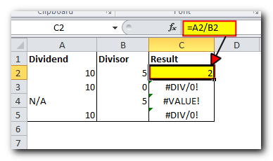
To avoid those errors, you can use the IFERROR function to catch and handle them in a way that works for you.
If there's an error, show a blank cell
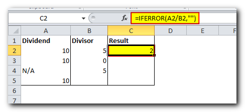
You can tell Excel to show a blank cell if an error happens by giving an empty string (“”) as the value for the value_if_error part of the formula. Here’s an example:
=IFERROR(A2/B2, “”)
In this case, if dividing A2 by B2 results in an error, Excel will show a blank cell instead
If error, then show a message
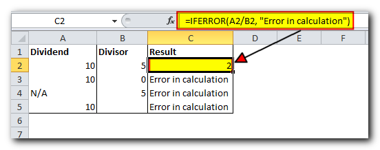
You can also display your own message instead of Excel’s standard error notation:
=IFERROR(A2/B2, “Error in calculation”)
5 things you should know about Excel IFERROR function
- The IFERROR function in Excel can handle all types of errors, such as #DIV/0!, #N/A, #NAME?, #NULL!, #NUM!, #REF!, and #VALUE!.
- Depending on what you put in the value_if_error part, IFERROR can replace the error with a custom message, a number, a date, a logical value, the result of another formula, or simply a blank cell (empty string).
- If the value you’re checking is a blank cell, Excel treats it as an empty string (“”), not an error.
- IFERROR was first introduced in Excel 2007 and is available in all later versions, including Excel 2010, 2013, 2016, 2019, 2021, and Excel 365.
- For Excel 2003 and earlier versions, you need to use the ISERROR function along with IF to handle errors. Here’s an example of how to do that.
IFERROR formula examples
The following examples show how to use IFERROR in Excel in combination with other functions to accomplish more complex tasks.
Excel IFERROR with Vlookup
A common use of the IFERROR function is to let users know when the value they’re searching for isn’t found in the data. You can do this by using IFERROR with a VLOOKUP formula, like this:
=IFERROR(VLOOKUP(...), "Value not found")
This way, if the VLOOKUP doesn’t find a match, it will show the message “Value not found” instead of an error.
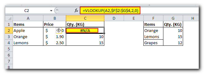
For your users’ piece of mind, wrap VLOOKUP in IFERROR and display a more informative and user-friendly message:
=IFERROR(VLOOKUP(A2, ‘Lookup table’!$A$2:$B$4, 2,FALSE), “Not found”)
The screenshot below shows this Iferror formula in Excel:

Nested IFERROR functions to do sequential Vlookups in Excel
When you need to run multiple VLOOKUPs based on whether the previous one worked or not, you can use IFERROR more than once by nesting them together.
For example, let’s say you have sales reports from different regional branches, and you want to find the amount for a specific order ID. Your order ID is in cell A2, and you want to search in three different sheets (Report 1, Report 2, and Report 3). You can use the following formula:
=IFERROR(VLOOKUP(A2,’Report 1′!A2:B5,2,0),IFERROR(VLOOKUP(A2,’Report 2′!A2:B5,2,0),IFERROR(VLOOKUP(A2,’Report 3′!A2:B5,2,0),”not found”)))
The result will look something similar to this:


IFERROR in array formulas
As you may know, array formulas in Excel are designed to carry out multiple calculations in a single formula. If you use an array formula or an expression that gives an array of values in the value argument of the IFERROR function, it will return an array of results for each cell in the specified range.
Here’s an example to explain:
Let’s say you have Total in column B and Price in column C, and you want to calculate the Total Quantity. You can do this using the following array formula, which divides each cell in the range B2
by the matching cell in the range C2, and then adds up the results:
=SUM($B$2:$B$4/$C$2:$C$4)
The formula works fine as long as the divisor range does not have zeros or empty cells. If there is at least one 0 value or blank cell, the #DIV/0! error is returned:
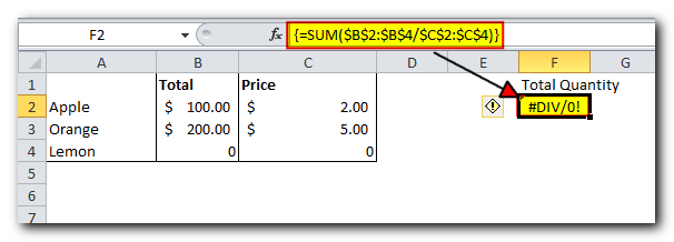
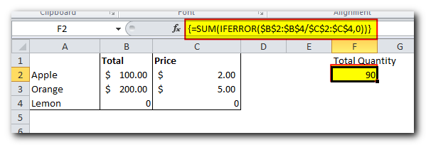
To fix the error, you can perform the division inside the IFERROR function like this:
=SUM(IFERROR($B$2:$B$4/$C$2:$C$4, 0))
Here’s what the formula does: It divides each value in column B by the corresponding value in column C for each row (100/2, 200/5, and 0/0), giving the results {50; 40; #DIV/0!}. The IFERROR function catches any #DIV/0! errors and replaces them with 0. Then, the SUM function adds up the values in the array {50; 40; 0}, and the final result is 90 (50 + 40)
IFERROR vs. IF ISERROR
Now that you see how simple it is to use the IFERROR function in Excel, you might wonder why some people still prefer using the combination of IF and ISERROR. Does it offer any benefits over IFERROR? The answer is no. Back in the older versions of Excel (like Excel 2003 and earlier), IFERROR didn’t exist, so using IF with ISERROR was the only way to catch errors. But in Excel 2007 and later, using IFERROR is just a simpler and quicker way to do the same thing.
For example, to catch VLOOKUP errors, you can use either of these formulas.
In Excel 2007 – Excel 2016
IFERROR(VLOOKUP(…), "Not found")
In all Excel versions:
IF(ISERROR(VLOOKUP(…)), "Not found", VLOOKUP(…))
Best practices for using IFERROR in Excel
By now, you know that the IFERROR function is the easiest way to catch errors in Excel and replace them with blank cells, zeros, or your custom messages. However, that doesn’t mean you should use error handling in every formula. The following tips can help you use it wisely:
- Don’t trap errors without a reason: Only use error handling when it’s necessary.
- Wrap the smallest part of the formula in IFERROR: Apply IFERROR only where it’s needed, not to the whole formula.
- Use specific error-handling functions when needed:
- Use IFNA or IF ISNA to catch only #N/A errors.
- Use ISERR to catch all errors except for #N/A.
This is how you can use the IFERROR function to manage errors in Excel. If you want to explore the examples mentioned in this tutorial, feel free to download our sample IFERROR Excel workbook. Thank you for reading, and I hope to see you on our blog next week!


