Index Match in Excel
Index Match in Excel are powerful tools for advanced lookups. They’re popular because they’re incredibly flexible. You can use them to search horizontally or vertically, perform two-way searches, find values to the left of your search criteria, handle case-sensitive searches, and even search using multiple conditions. If you want to improve your Excel skills, mastering INDEX and MATCH is essential. Below, you’ll find numerous examples to help you grasp how they function.
This article demonstrates how to use INDEX and MATCH together for searching in Excel. It walks you through each step, starting with INDEX, then explaining MATCH, and finally showing you how to combine them to conduct a two-way search
Table of Contents
The Index Function
The INDEX function in Excel is both versatile and powerful, often featured in advanced formulas. But what does INDEX actually do? In simple terms, it retrieves a value from a specific location within a range. For example, suppose you have a table listing planets in our solar system (as shown below), and you want to find the name of the 4th planet, which is Mars. You can use INDEX to accomplish this
Syntax:- =INDEX(B3:B11,4)
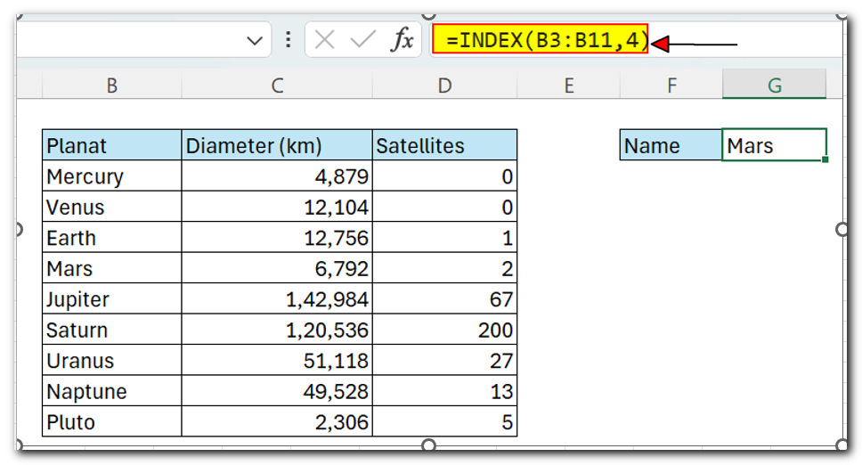
INDEX returns the value in the 4th row of the range.
If you want to find out the diameter of Mars using INDEX, you can specify both a row number and a column number within a larger range of data. The INDEX formula below shows how to do this using the entire range B3:D11, where we specify row 4 and column 2
Syntax:- =INDEX(B3:D11,4,2)
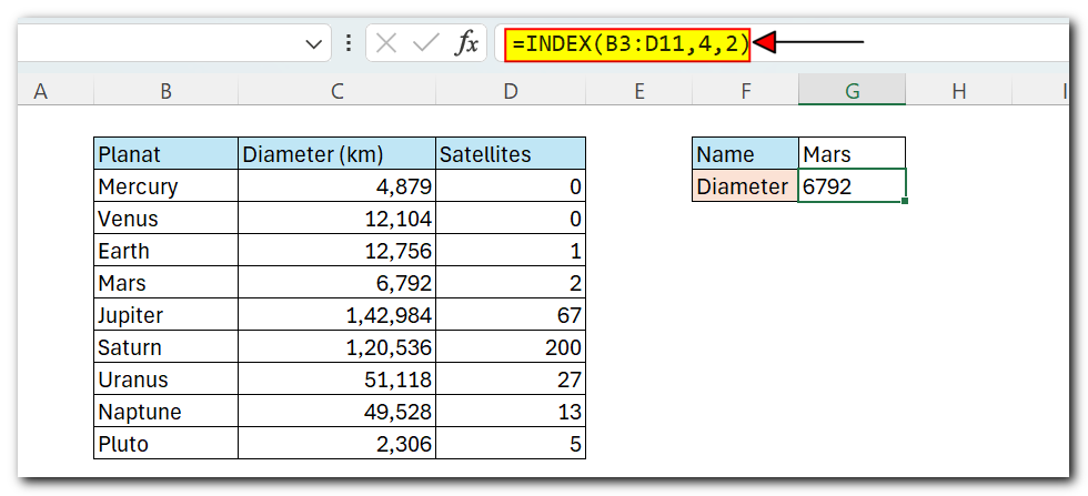
INDEX retrieves the value located at row 4, column 2.
In simple terms, INDEX fetches a value from a specific spot in a group of cells using numerical positions. If the group is arranged in a single row or column, you provide only a row number. If it spans two rows or columns, you specify both row and column numbers.
Now, you might be wondering, ‘Why does this matter? How often do we actually know where something is in a spreadsheet?’
Exactly! We often need a way to find the exact position of what we’re looking for
Enter the MATCH function
The Match Function
The MATCH function has one main job: to find where an item is in a group. For instance, we can use MATCH to locate where the word “Monday” is in this list of fruits, like this:
Syntax:- =MATCH(“Monday”,B3:B9,0)
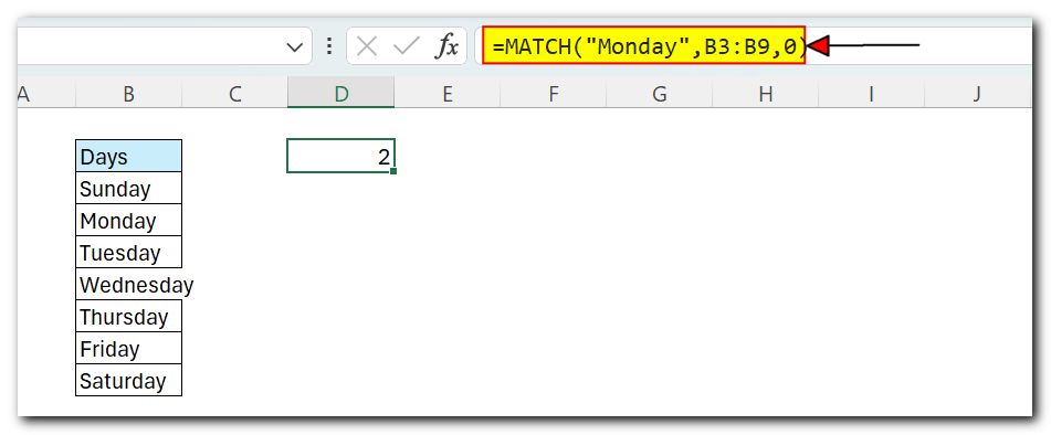
MATCH returns 2, since “Monday” is the 2nd item. MATCH is not case-sensitive.
MATCH doesn’t care if a range is horizontal or vertical, as you can see below:
Syntax:- =MATCH(“Monday”,B2:H2,0)

Using a horizontal range, MATCH returns 2, yielding the same result.
Note: the final argument in the MATCH function is match_type. This setting is significant because it determines whether the matching is exact or approximate. In most cases, you should use zero (0) to ensure exact matching behavior. The default match_type is 1, which signifies approximate matching, so it’s important to specify the desired value.
Index and Match together
Now that we’ve covered the basics of INDEX and MATCH, how do we combine the two functions in a single formula? Consider the data below, a table showing a list of salespeople and monthly sales numbers for three Days: Sunday, Monday and Tuesday
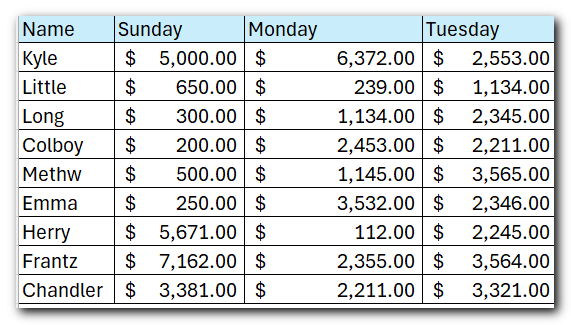
Understanding the Data Structure:
- Column A: Salespeople names (A1 to A10)
- Column B: Sunday sales (B1 to B10)
- Column C: Monday sales (C1 to C10)
- Column D: Tuesday sales (D1 to D10)
Using Index and Match
- INDEX function is used to return a value from a specified range based on a row and column number.
- MATCH function is used to find the position of a value within a range.
Syntax & discription
=INDEX(range, MATCH(lookup_value, lookup_range, match_type), column_number)
- range: The entire range of sales data (including all salespeople and all Days)
- lookup_value: The specific salesperson’s name you are looking for (e.g., “Salesperson EMMA”).
- lookup_range: The range where the salespeople names are located (Column A).
- match_type: 0 (exact match)
Example:
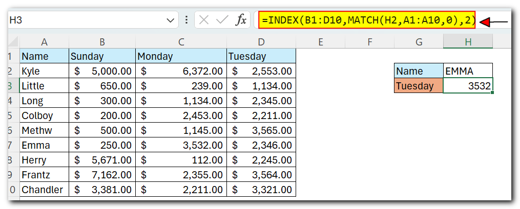
Let’s say you want to retrieve the sales number for a specific salesperson (let’s call it “Salesperson A”) for the month of Monday Assuming your data starts from A1
the formula would be
=INDEX(B1:D10, MATCH(H2, A1:A10, 0),2)
2 Ways lookup with Index and Match
Earlier, we used the MATCH function to find the row number dynamically but hardcoded the column number. To fully automate the formula and retrieve sales for any salesperson in any month, we can use MATCH twice – once to find the row position and once to find the column position.
From the examples above, we know MATCH works fine with both horizontal and vertical arrays. That means we can easily find the position of a given month with MATCH. For example, this formula returns the position of Tuesday, which is 3:
=MATCH(“Tuesday”,B2:D2,0) // returns 3
But of course, we don’t want to hardcode any values, so let’s update the worksheet to allow the input of a month name and use MATCH to find the column number we need. The screen below shows the result

Syntex:
=INDEX(B2:D10,MATCH(H2,A3:A11,0),MATCH(H3,B1:D1,0))
The first MATCH formula returns 6 to INDEX as the row number, and the second MATCH formula returns 3 to INDEX as the column number. Once MATCH runs, the formula simplifies to:
=INDEX(B2:D10,6,3)
and INDEX correctly returns $ 2,346.00 the sales number for Emma on Tuesday.
Left Lookup
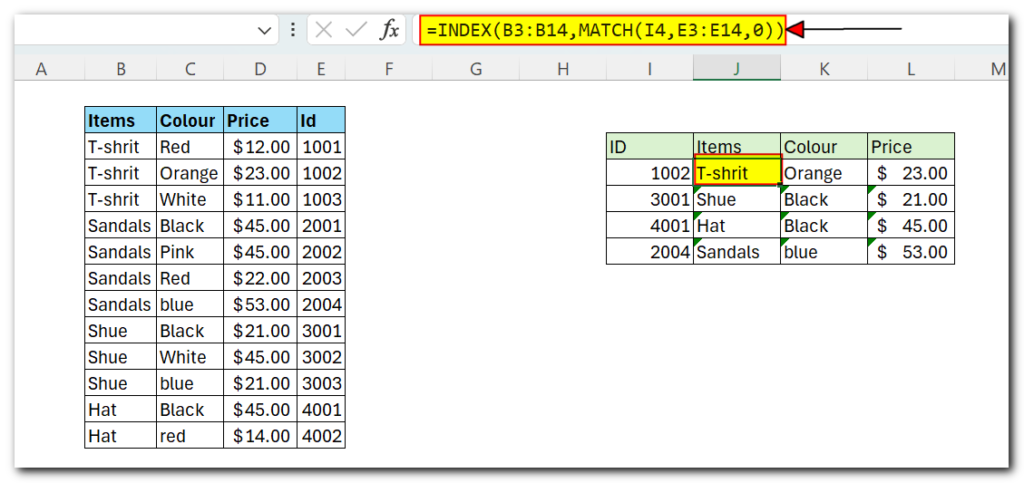
One big advantage of using INDEX and MATCH instead of VLOOKUP is that it allows you to do a ‘left lookup’. This means you can look up information based on a key even if the key column is to the right of the data you want to find, as shown in the example below
Index Match with multiple Criteria
Excel can be challenging when you need to find something based on multiple conditions, like matching more than one column simultaneously. One effective way to solve this is by using Boolean logic. This technique treats TRUE and FALSE values like 1s and 0s. Below, you can see how we apply this approach with INDEX and MATCH to find a price using three criteria: Item, Color, and Size.

Case-sensitive lookup
The MATCH function doesn’t pay attention to whether letters are uppercase or lowercase. But if you want to do a lookup that does care about case (like matching ‘APPLE’ exactly with ‘APPLE’ and not ‘apple’), you can use the EXACT function with INDEX and MATCH, as demonstrated below:

Closest Match
Another way to see how INDEX and MATCH can be useful is when you need to find the closest match. In the example below, we use the MIN function along with the ABS function to set up a value to look for and a range to search within the MATCH function. This way, MATCH finds the smallest difference. Then, we use INDEX to get the corresponding result from column B

Index and Xmatch
The latest Excel now has the XMATCH function, which is an improved version of MATCH. XMATCH does what MATCH does — it looks up and gives you a position number. It works for both vertical and horizontal ranges, and it can find exact or close matches. Plus, you can use wildcards like * or ? to find partial matches. But XMATCH has some extras that make it even better
5 main difference between Xmatch and Match
- XMATCH looks for an exact match by default, while MATCH usually looks for an approximate match.
- XMATCH can find the next larger or smaller item in a list.
- XMATCH can search in reverse order, from the last item to the first.
- XMATCH doesn’t need values to be sorted when looking for an approximate match,
- XMATCH can use a binary search method, which is faster and more efficient for large datasets.


