How to Use Filter in Excel
Table of Contents
Filter in Excel is an essential tool that helps to display relevant data. It eliminates the irrelevant entries temporarily from the view. This tool filters data according to the criteria to help analyze the critical data points
This article talks about what filtering in Excel means, why it’s helpful, how to do it, and gives some examples
How to add Filter in Excel?
To use Excel AutoFilter correctly, your data should have a top row with names for each column
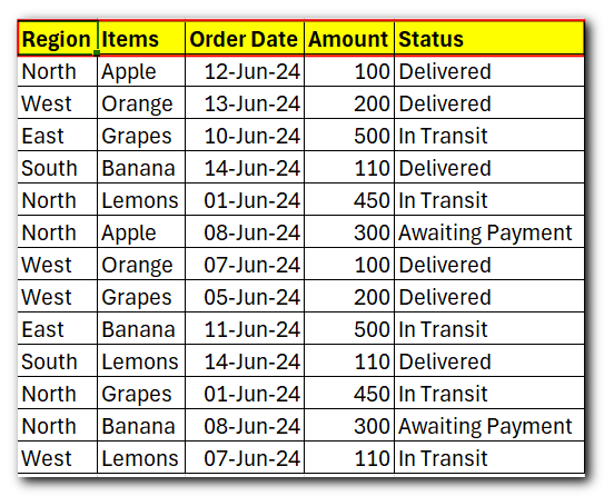
Once you have the column headings in place, select any cell within your dataset, and you can use one of the following methods to insert a filter.
3 Ways to add Filter in Excel
1. Go to the Data tab > Then go to Sort & Filter group and click the Filter button to apply a filter to your data.
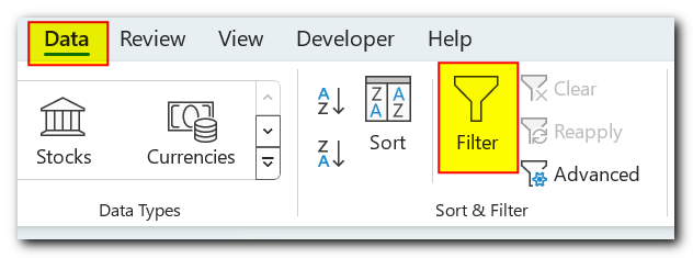
2. On the Home tab, in the Editing group, click Sort & Filter, and then click Filter to apply a filter to your data.
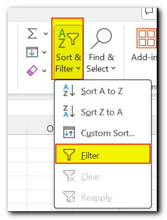
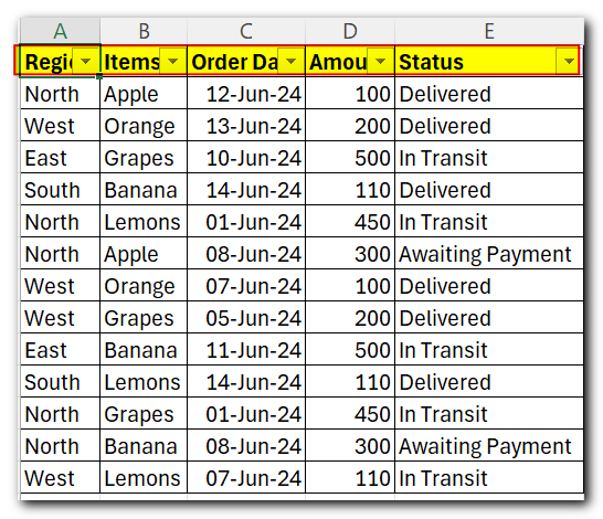
3. Use the Excel Filter shortcut to quickly turn filters on or off: press Ctrl+Shift+L or Alt D+F+F. Whichever method you choose, drop-down arrows will appear in each of the header cells. Explore more shortcut keys
What is Filter in Excel ?
Excel Filter, also called AutoFilter, quickly shows only the information you want to see and hides the rest. You can filter rows in Excel sheets by their values, appearance, or specific rules you set. After applying a filter, you can apply multiple things like (manipulate, copy, edit, create charts, or print only) the visible rows without affecting the entire list.

Difference between Excel Filter vs Excel Sort
In addition to many ways to filter data, Excel’s AutoFilter
lets you sort data in different ways for each column:
- For text values: You can sort from A to Z, from Z to A, and by colour
- For numbers: You can sort from smallest to largest, from largest to smallest, and by colour
- For dates: You can sort from oldest to newest, from newest to oldest, and by colour
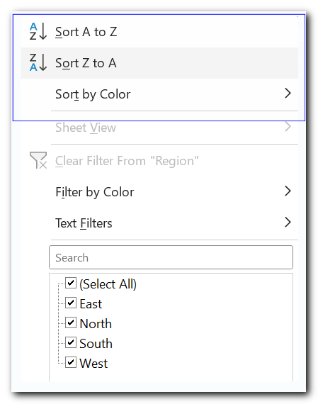
The difference between sorting and filtering in Excel is as follows:
- When you sort data in Excel, the entire table is rearranged, for example alphabetically or from the lowest to the highest value. However, sorting does not hide any entries, it only puts the data into a new order
- When you filter data in Excel, only the entries you want to see are displayed, and all irrelevant items are temporarily removed from view
How to apply Filter in Excel ?
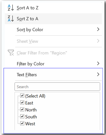
When you see a drop-down arrow in a column heading in Excel, it means filtering options are available but not active yet. If you hover over the arrow, a screen tip shows “Showing All”.
To filter data in Excel, follow these steps:
- Click the drop-down arrow for the column you want to filter.
Uncheck the “Select All” box to quickly remove all selections..
Check the boxes next to the data you want to see, then click OK.
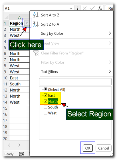
Done! Now the filter is applied to column A, so you’ll only see data for East and North regions, hiding all others temporarily.
The drop-down arrow in the filtered column changes to a Filter button , and when you hover over it, a screen tip shows which filters are active.
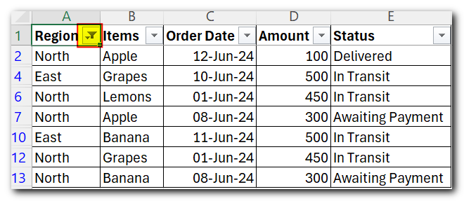
Filter multiple columns
To apply Excel filters to multiple columns, simply follow the same steps for each column you want to filter.
For instance, let’s say we want to see only sales of Apples in the East and North regions. When you apply filters to multiple columns in Excel, a filter button will show up in each of those columns that have filters applied.

In Excel Online, the View menu keeps things pretty simple. You can do basic stuff like freezing panes and showing gridlines. But if you’re used to the desktop version, you’ll notice some things are missing, like page layout, custom views, and macros. That’s just because online versions have some limits compared to desktop ones.
In Excel Online, the View menu keeps things pretty simple. You can do basic stuff like freezing panes and showing gridlines. But if you’re used to the desktop version, you’ll notice some things are missing, like page layout, custom views, and macros. That’s just because online versions have some limits compared to desktop ones.
How to use Filter in Excel using text filters?
In addition to the basic filtering options, we talked about earlier, AutoFilter in Excel offers advanced tools that let you filter different types of data, like text, numbers, and dates, exactly how you need them.
Text Filter Data
When you need to filter a text column for something very specific, Excel offers advanced options through Text Filters
- Filter cells that start with or end with certain characters
- Filter cells that exactly match or do not match specified characters
- Filter cells that contain or do not contain specific characters or words anywhere in the text.
Once you apply a filter to a column with text, these Text Filters will automatically show up in the AutoFilter menu similar to shown below:
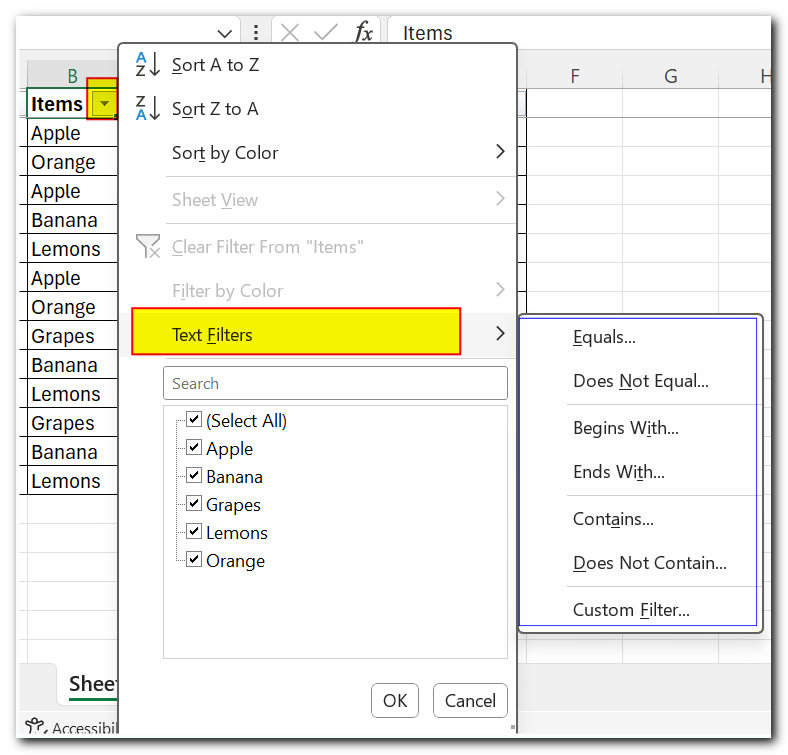
For example, if you want to filter out rows that contain “Banana,” follow these steps
- Click the drop-down arrow in the column heading, then point to Text Filters
- From the drop-down menu, choose the filter you want (like “Does Not Contain…” in this case).
- A Custom AutoFilter box will appear. In the box next to the filter, type the text or choose from the list.
- Click OK when you’re done
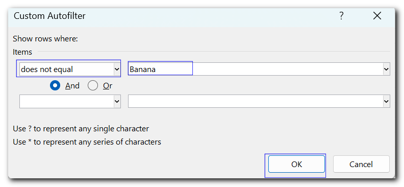
As a result, all rows containing “Banana,” such as “Green bananas” and “Goldfinger banana,” will be hidden
Filter Column with 2 Criteria
To filter data in Excel with two text criteria, follow the steps for the first criterion, and then:
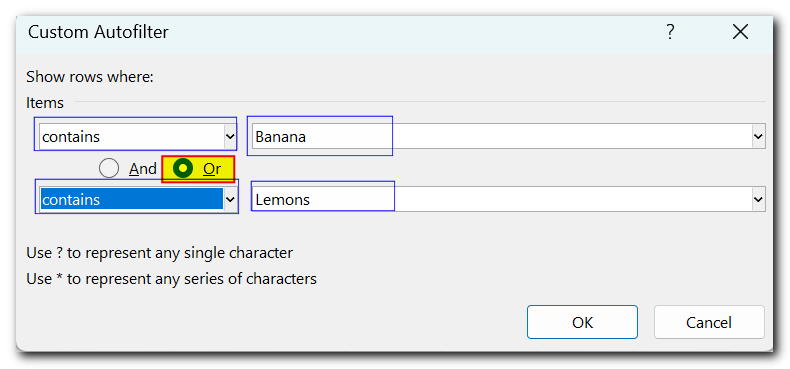
- Check the “And” or “Or” radio button depending on whether both or either criterion should be true
- Select the comparison operator for the second criterion and enter the text value in the box next to it
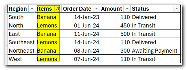
For example, this is how you can filter rows that contain either “Bananas” or “Lemons”:
How to create Filter in Excel with Wildcard characters?
If you can’t remember the exact search term or want to filter rows with similar information, you can create a filter using one of the following wildcard characters
Wildcard character | Description | Example |
? (question mark) | Matches any single character | Gr?y finds “grey” and “gray” |
* (asterisk) | Matches any sequence of characters | Mid* finds “Mideast” and “Midwest” |
~ (tilde) followed by *, ?, or ~ | Allows filtering cells that contain a real question mark, asterisk, or tilde. | What~? finds “what?” |
How to Filter number in Excel?
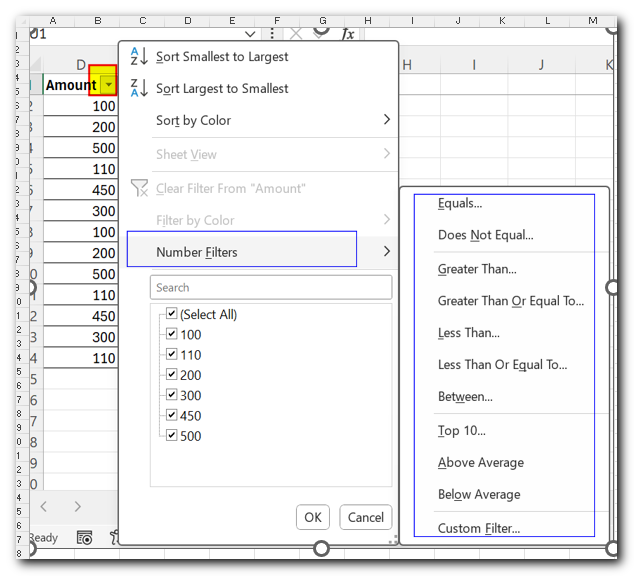
Excel’s Number Filters let you work with numeric data in many ways, such as
- Filtering numbers that are equal to or not equal to a specific number
- Filtering numbers that are greater than, less than, or between certain values
- Filtering the top 10 or bottom 10 numbers
- Filtering numbers that are above or below the average
The screenshot below shows all the different number filters you can use in Excel.
Note: If the number filter is applied, the selected row must contain only numeric values
For instance, if you want to filter orders between 200 and 300, follow these steps:
- Click the auto filter arrow in the column header and choose Number Filters
- Select “Between…” from the options
- In the Custom AutoFilter box, enter the lower and upper values. Excel usually suggests using “Greater than or equal to” and “Less than or equal to” by default. If you prefer, you can change these to “Greater than” and “Less than” to exclude the boundary values
- Click OK when you’re done
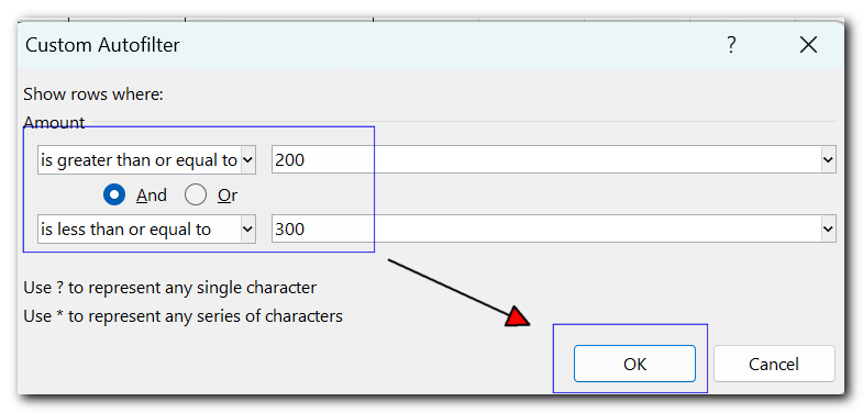
As a result, you’ll only see orders that are between 200 and 300.

How to Filter Date in Excel
Excel’s Date Filters offer a wide range of options to help you quickly and easily filter records for specific time periods
By default, Excel’s AutoFilter organizes dates in a column by year, month, and day. You can expand or collapse these groups by clicking the plus or minus signs next to each group. When you select or clear a higher-level group, it affects all nested levels. For example, clearing the box next to “2024” hides all dates within that year.
Date Filters allow you to show or hide data for a specific day, week, month, quarter, or year. You can also filter data before or after a certain date, or between two dates. The screenshot below shows all the available date filter options.
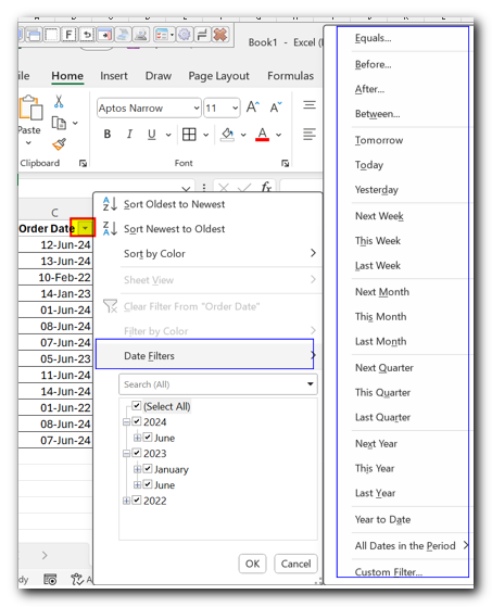
In most cases, filtering by date in Excel is as easy as a single click. For example, to filter rows with records from the current week, just go to Date Filters and click on “This Week.”
If you choose the Equals, Before, After, between operators, or Custom Filter, you’ll see the familiar Custom AutoFilter dialog box where you can set your criteria
How to Filter by colour in Excel ?
If your worksheet data is formatted manually or using conditional formatting, you can also filter by colour
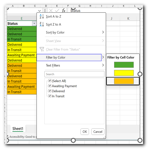
Clicking the auto filter drop-down arrow will show “Filter by Colour,” with options based on the formatting applied to each column
- Filter by cell colour
- Filter by font colour
- Filter by cell icon
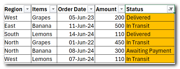
For example, if you formatted cells in a given column with 3 different background colors (green, Yellow and orange) and you want to display only orange cells, you can get it done in this way:
- Click the filter arrow in the header cell, and point to Filter by Color
- Click the desired color – orange in this example
only values formatted with the orange font colour are visible and all other rows are temporarily hidden
How to Filter in Excel with search ?
Starting from Excel 2010, the Filter interface includes a search box. This makes it easier to navigate large datasets by allowing you to quickly filter rows that contain specific text, numbers, or date
Suppose you want to view the records for all “east” regions. Just click the autofilter dropdown and start typing the word “east” in the search box. Excel Filter will immediately show you all items that match the search. To display only those rows, either click OK in the Excel AutoFilter menu, or press the Enter key on your keyboard
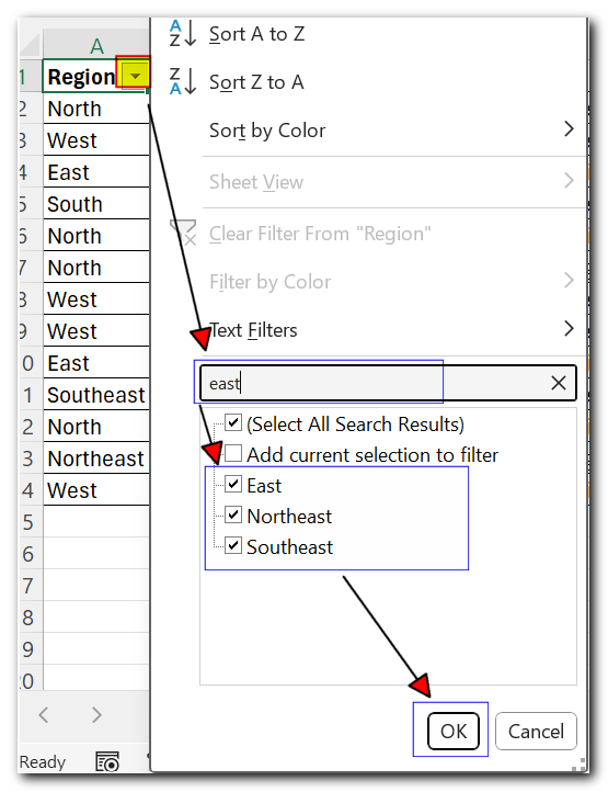
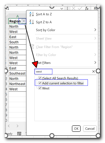
To filter multiple searches, apply a filter according to your first search term as demonstrated above, then type the second term, and as soon as the search results appear, select the Add current selection to filter box, and click OK. In this example, we are adding “west” records to the already filtered “east” items
Re-apply a Filter after changing the data
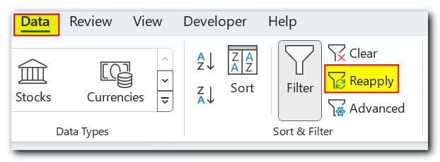
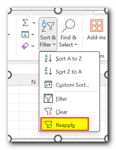
When you edit or delete data in filtered cells, Excel AutoFilter does not update automatically to reflect the changes. To re-apply the filter, click any cell within your dataset, and then either:
- Click Reapply on the Data tab, in the Sort & Filter group
2. Click Sort & Filter > Reapply on the Home tab, in the Editing group
How to clear Filter ?
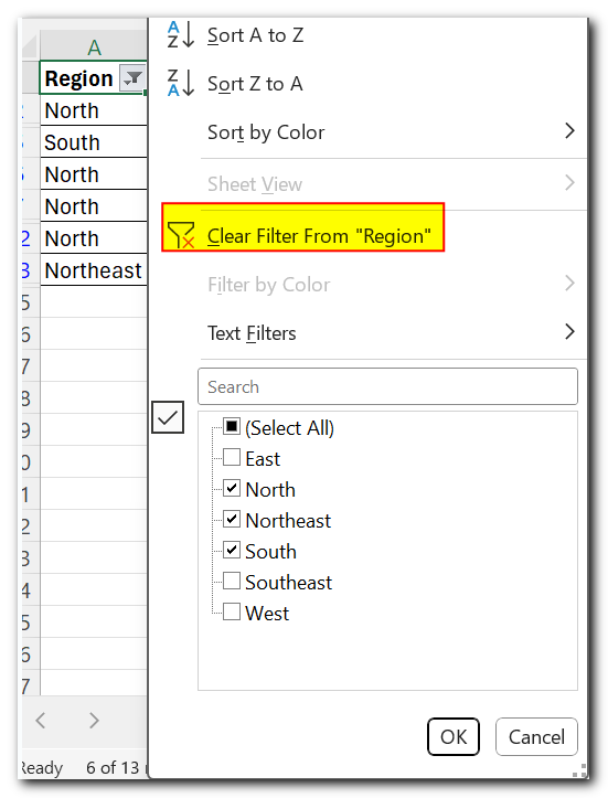
After applying a filter to a certain column, you may want to clear it to make all information visible again or filter your data in a different way.
To clear a filter in a certain column, click the filter button in the column’s header, and then click Clear Filter from <Column name>:
How to remove Filter in Excel ?
To remove all filters in a worksheet, do one of the following:
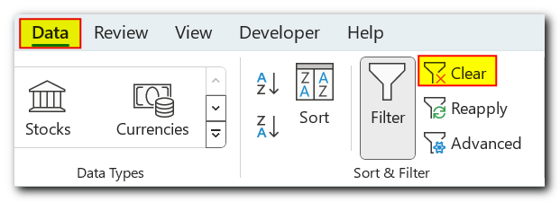
- Go to the Data tab > Sort & Filter group, and click Clear
- Go to the Home tab > Editing group, and click Sort & Filter > Clear
