Join Multiple Excel Tables with Power Query
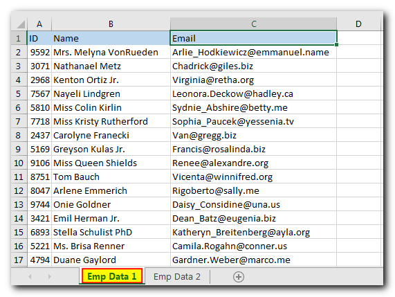
Introduction
The second sheet has got other information of the employee such as Job Title, Department, City, State, Postal Code and Country.
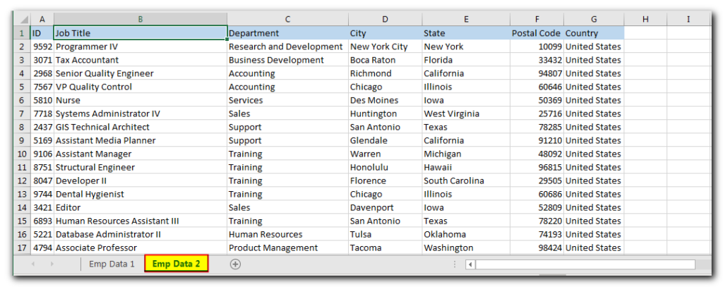
Note: The ID column which you can also consider as Employee ID is common in both the sheets.
What we want to achieve?
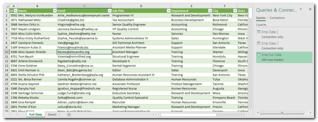
We want to create a new view in Excel which has all the information of the employees from both the sheets.
Steps to join two data sets using Power Query:
Let’s start from a new Excel file
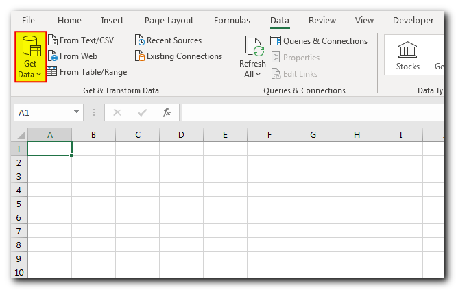
From the Data ribbon, click on Get Data button
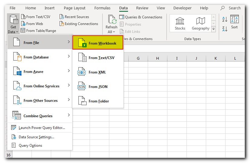
As our data is in Excel file; hence we will select “From Workbook” option under “From File”
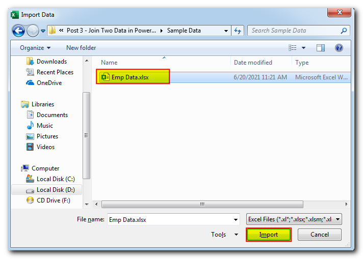
Select the file which contain the employee data and click on ‘Import’ button
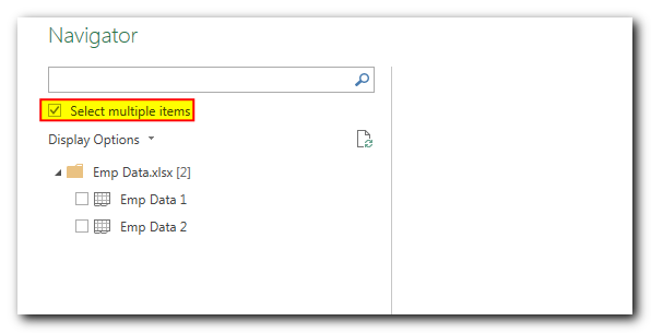
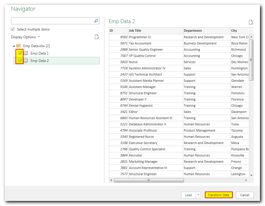
As our data is spread across two different sheets so we need to check the “Select multiple items” checkbox on the query window
Now let’s select both the sheets and click ”Transform Data” button
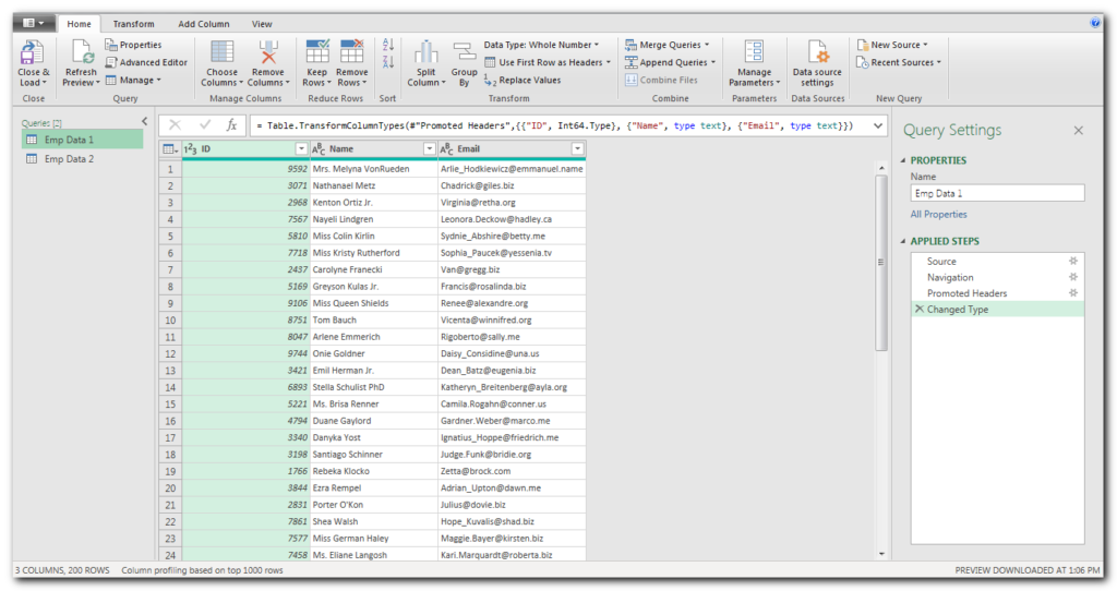
In few moments, Power Query Editor should get loaded
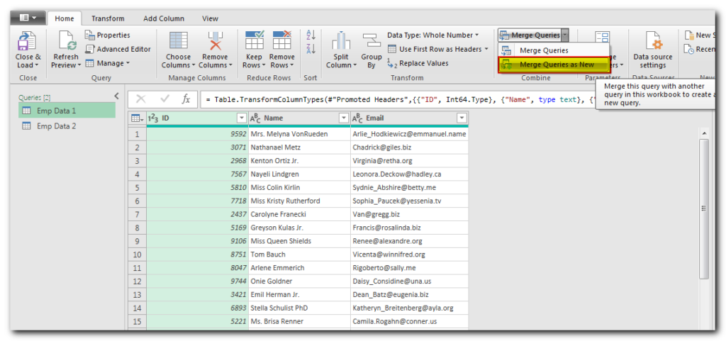
The next task is to merge both the queries and create a combined query. To do this, we need to select “Merger Queries and New” under Home ribbon.
In the merge dialog box, we need to select the tables which we want to merge. Here we have selected “Emp Data 1” and “Emp Data 2”
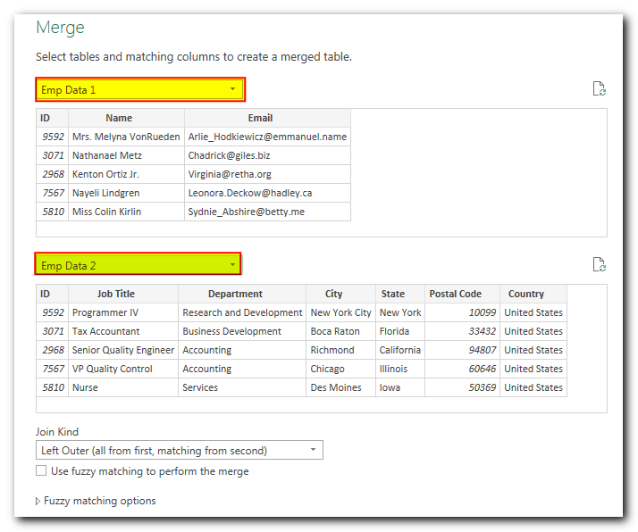
Next, we need to select the column which will be used to join both the tables together. You should select a column which is available in both the tables. In our case it is ID column which is available in both tables.
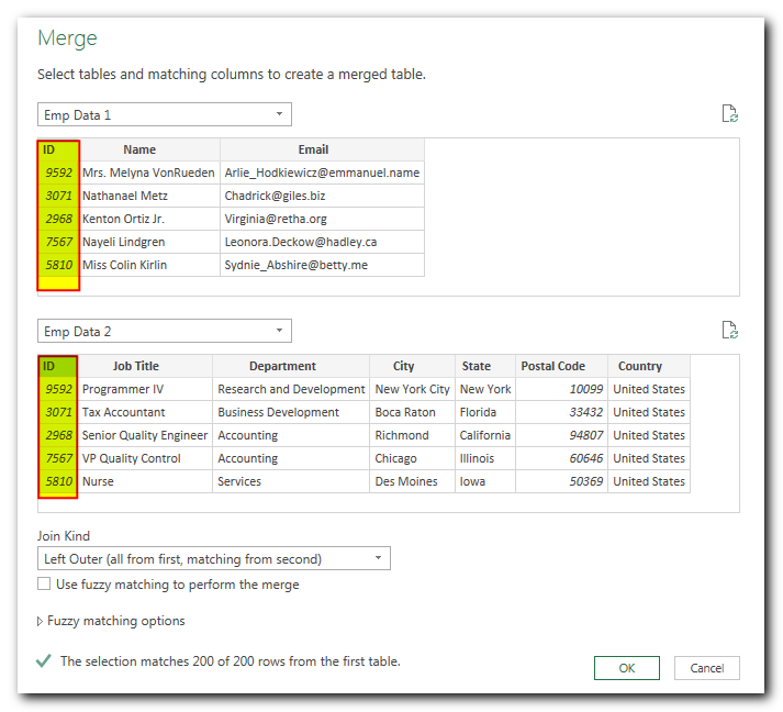
The last step to merge the table is to select the join type. Here we will be selecting Left Outer join which means all the records from “Emp Data 1” and only the matching records from “Emp Data 2” will be included in the result.

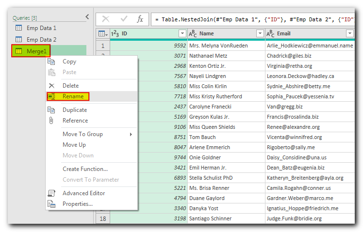
The query is created, let’s rename it to “Emp Full Data”
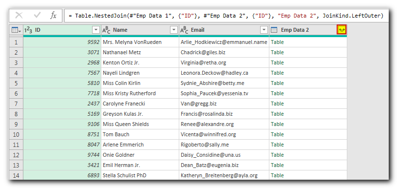
We need to expend “Emp Data 2” field to get the columns from second table (in our case the columns from “Emp Data 2” sheet. Let’s click on expend button
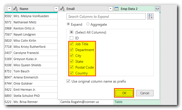
Let’s select all the columns apart from ID (as ID column is already available in Emp Data 1) and click on OK button
You will notice that the selected columns are added in the Query
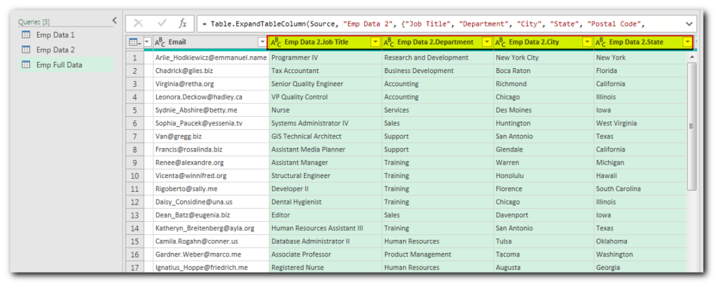
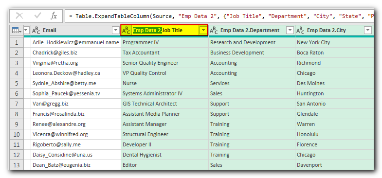
Now we need to remove the table name (Emp Data 2) from the newly added column names
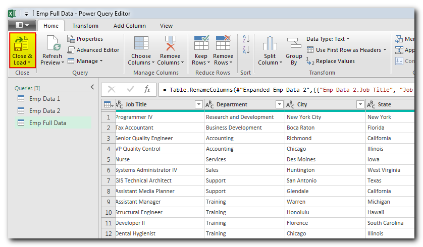
Once done, we will click on “Close & Load” button under Home ribbon
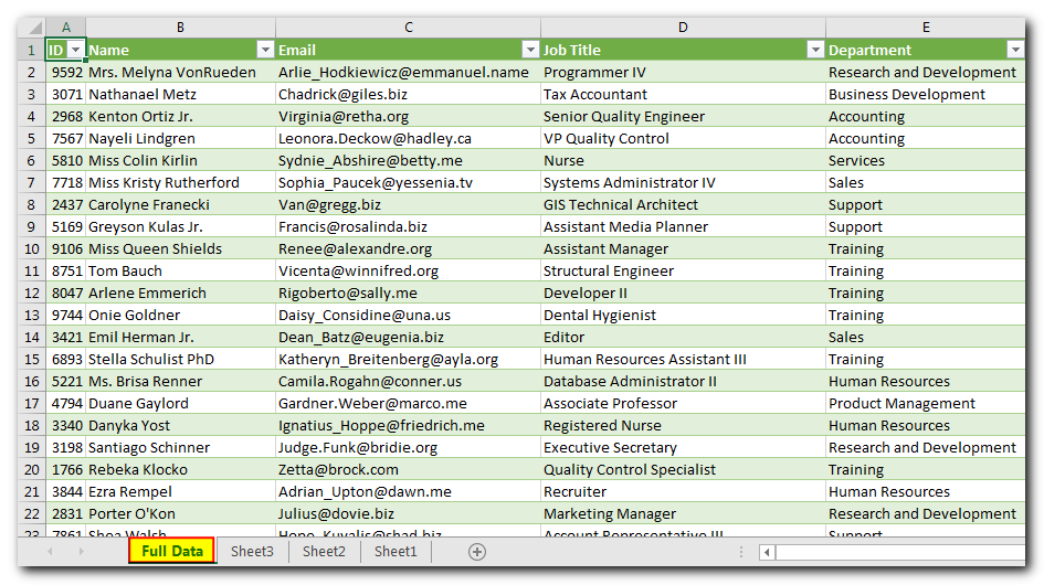
Our query is ready. You will notice that 3 new sheets have been added in the file
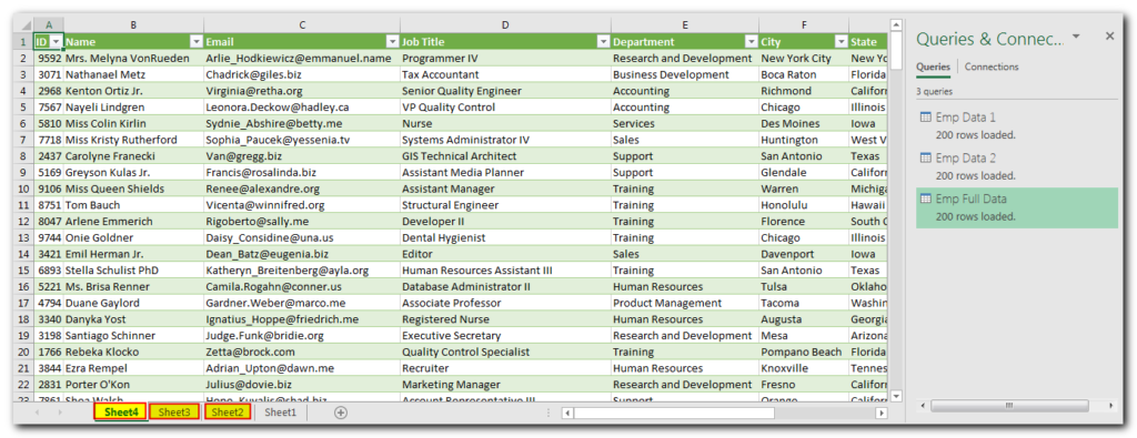
In our case “Sheet4” contains the view that we were looking for. Let’s rename it to “Full Data”
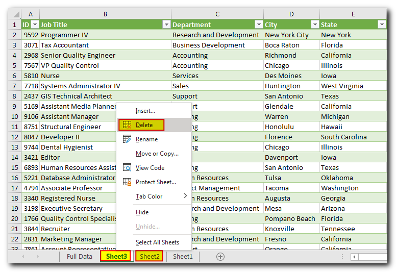
Sheet3 and Sheet2 contains data from “Emp Data 1” and “Emp Data 2”. As our main purpose was to get combined view from both the sheets, so let’s delete them.
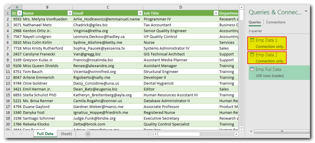
You will notice that Query type is changed to “Connection only” which is fine.
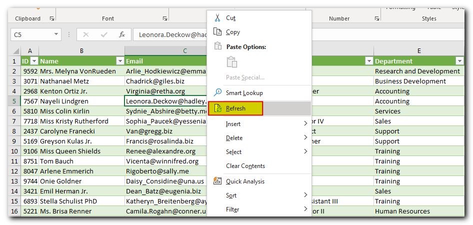
In future, if there is new data is added in the Excel file then you just need to refresh the query to get latest data
